1. Introduction

The digital elevation model (DEM) plays an important role in geographic information system (GIS). The applications of DEM integrating with additional information can range many fields such as hydrological studies[1-4], soil investigation and modelling[1-5] and natural disaster studies for flooding[6-9]. However, any reports related to modelling bushfires in landscape using DEM have not been found. The main difficulties in this field are those:

• No necessary information about observed objects in landscapes can be acquired from DEM,

• Lack in necessarily understanding how bushfire spreads in landscapes.

The efforts without using DEM can be found from some previous works. Several researchers[10-13] proposed a series of abstract mathematic models and performed some small scale experiments as a main point of studying.

However, the achievement made by those researches could not represent large scale bushfires[14].

Consequently, a new idea in studying the large scale bushfire is to be proposed in this paper. The novel approach is an interdisciplinary study. It combines and utilizes the unique features of DEM and the corresponding satellite imagery and then applies some knowledge from other disciplines such as meteorology, combustion and transport phenomena to resolve the following drawbacks and main difficulties:

DEM fails to supply the information of distribution of vegetation besides elevation,

Satellite imagery only offers two-dimensions (2-D) based information,

How bushfire spreads in landscapes (affected by geometric shape of terrain),

How the pollutant ( thus smoke) spatially disperses,

How smoke impact upon the surface,

How to estimate the amount of released energy and mass during bushfire spread,

How the bushfire spread is affected by solar radiation (spread velocity is different at day and night time),

And so on

Objectives and scales of research

Nevertheless, the scale in this paper is only to focus on

1. How the distribution of vegetation is classified in the remote sensing imagery.

2. How the classified data from the remote sensing imagery is transferred into DEM.

3. How to determine the direction of bushfire spread combining the remote sensing and DEM.

4. How to create a linear index in a matrix.

5. How to convert a vector point in a coordinates of DEM and generate linear indices.

6. How to model a simple case of bushfire spread in landscape based on DEM for further approaches.

7. How to display the information gained from modeling in DEM into original remote sensing imagery reversely.

Meanwhile, some basic concepts and techniques used in the digital image processing and the geomorphology integrating with the features of DEM are to be included.

2. Methodology

2.1. On Identifying Substances in Remote Sensing Imagery

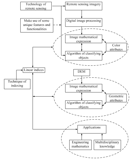
Because this research is based on remote sensing imagery and digital elevation model (DEM). Some concepts related to digital image processing are briefly mentioned as follows. They may be helpful in understanding the procedure that how the data are captured by sensors and stored in the form of digital imagery, why identifying objects must be classified and how to perform it by means of creating new techniques.

Principle of Remote Sensing

Remote sensing is a method of acquiring information about an object or phenomenon without physically contacting. It consists of a series of process before information is obtained (see Figure 1 ). The electromagnetic wave, energy and spectrum play an important role in transferring signal, imaging, analysing object and phenomenon. The platform usually is a satellite or aircraft. Sensors consist of several devices having different functionalities. The digital imaging happens in a charge-coupled device (CCD) to catch each incoming photon and digitally expose it in a matrix-like linear CCD array, and then a digital image is formed[15].

Figure 1. principle of remote sensing

The information from a narrow wavelength range is gathered and stored in a channel of satellite, also named as a band. In the Landsat case, there are seven bands (see Figure 2). Hence, they have discrete wavelength ranges and belongs to multispectral imaging.The information in bands is combined and displayed digitally by the three primary colors (Red, Green and Blue) (see Figure 3 ). According to the definition of Commission internationale de l'éclairage (CIE) about color, three visible primary colors have different wavelengths, they illustrate in Figure 4. The sensors are sensitive to light sources, which can make up of different mixtures of various wavelengths. In the digital image processing, the RGB tube is often used. The RGB tube in Figure 3 illustrates how the variation of color with the proportion of three components. The white color (light) appears when the ratio of three components is even. However, the different mixing colors representing different substances in a remote sensing imagery (e.g. Figure 8 ) are also characterized by other corresponding attributes such as Hue, Saturation and Intensity (see Figure 5 ). All colors have those attributes. The HIS space consists of a vertical intensity axis and the locus of color points which lie on a plane perpendicular to the intensity axis. The color points are arbitrary, that means any colors inside plane are not pure. Behind this fact, it implies that the incoming light has a mix of frequencies or wavelengths for any color points on the plain. For a specific hue (its angle ranges between 0° and 360°), increasing saturation is a process of purifying the color. The digital gray level is also presented by moving the plain up and down digitally. The HIS and RGB space can be converted mutually. For instance, the image captured by Landsat in Figure 8 becomes Figure 6 after normalized conversion. This treated image indirectly indicates how the devices installed in the satellite work and several potential working mechanisms and correlations.

In order to classify burning and smouldering zone in the remote sensing imagery, of importance is how identify the substances at the surface of Earth, which appear in one digital image. The most popular manner is using multispectral imaging or hyperspectral imaging based on the spectrum of electromagnetic radiation (see Figure 4). Bushfire spread along Australia east coast captured by Aqua MODIS in Figure 7 and the landscape in Victoria, Australia captured by Landsat in Figure 8 used the technique of multispectral imaging. As a result, the multispectral image is able to be read and dealt with as a RGB image in the image processing.

Spectral Signature of Substance

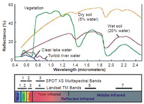Figure 2. typical spectral reflectance curves for vegetation, soil and water[16]

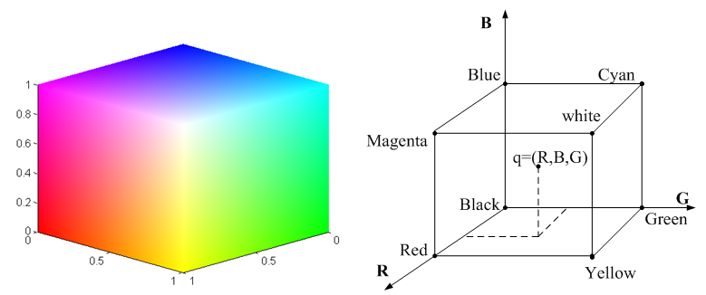Figure 3. RGB tube and RGB space

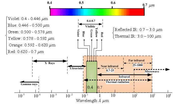Figure 4. the spectrum of electromagnetic radiation (redraw it based on[17-18])

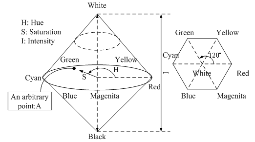Figure 5. relationships between RGB space and HIS space

Figure 6. HIS space-based remote sensing imagery Identify Substances

Various materials on the surface of the earth have spectral different reflectance characteristics[19]. There are three forms of interaction that can take place when energy strikes, or is incident upon the surface. They are absorption, transmission and reflection. The total incident energy interacts with the surface in one or more of these three ways.

For different substance has different spectral reflectance. Typical spectral reflectance curves for vegetation, soil and water are shown in Figure 2. These spectral signatures of substance are easily to distinguish substances at the surface. For instance, fire, smoke, ocean, lake, soil, vegetation and so on in Figure 7 and Figure 8 are easily to be distinguished by means of unique spectral signature of substance. Those typical spectral signatures are also to be used as criteria in creating an algorithm of classifying objects and assessing whether the result is satisfactory or not.

Limitations of Spectral Imaging in Application

Because the multispectral imaging only extracts several bands, it is not fine enough. In dealing with complicated cases, it may rely on hyperspectral imaging. Each pixel in an image made by the hyperspectral imaging has full spectral information with imaging narrow spectral bands over a contiguous spectral range.

However, the hyperspectral imaging still has several limitations. A typical problem is a lot of cost in dealing with its data. In the practical application, in the case of investigating bushfire, it fails to effectively detect the exact temperature of bushfire because of influence of smoke (CO₂ can absorb a lot of energy) and detect what amount of particles in smoke mixture per unit volume.

For such limitations, in fact, it is impossible to be resolved by the technology of remote sensing itself.

A dynamic process such as bushfire spread, flood happen on the earth may belong to the domain of engineering. Although a dynamic process may be able to model by a group of parameters, the most difficulty for modelling and forecasting is to find accurate value for each parameter, on the other hand, those values are impossible to be gained through a series of large-scale experiments, for example, bushfire. The best way of obtaining the values for those parameters may be by means of the technology of remote sensing.

Therefore, in this research, to know more information of bushfire spread and smoke dispersion, some necessarily modellings are required by combining the captured information from the remote sensing imagery and other disciplinary knowledge.To do so, the remote sensing imagery captured by Landsat is preferred to choose as a platform for modelling.

Figure 7. Aqua MODIS image was acquired on September 22, 2003[20]

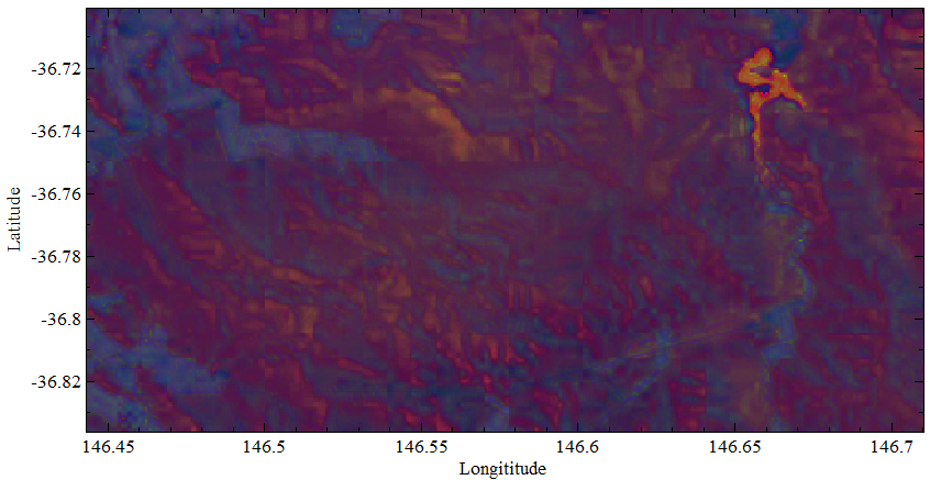
Figure 8. selected landscape of remote sensing imagery for modeling

2.2. On Further Development of Remote Sensing Imagery Integrating with Digital Elevation Model

Figure 9. schedule graph of further development integrating remote sensing imagery with DEM

In the preceding sections, some issues relative to the remote sensing imagery were briefly mentioned. The focus at this stage should be located onto how to model bushfire and even discover new techniques in the development of GIS. The further approach is based on the scheme shown in Figure 9, which continues from the tasks shown in Figure 1, but differs from them especially at final steps.

The new development has many potential opportunities to find out some new research manners and results which are impossible to be performed in some fields by means of traditional research methods including technology of remote sensing. This new approach is mutual benefit.

In this case, up to this point, the attempt is transferring the information from satellite imagery into three-dimensional DEM. This is the most important procedure. However, each observed and indexed object is also related to some unique properties owned by its individual system. In the following sections, the relevant properties are briefly introduced separately so as to know what a sort of properties is also linked during data transfer so as to provide more information for comprehensively modelling bushfire and enlarge the range of application in another development as well.

2.3. Concept of Processing Digital Image

A Digital Image as a Matrix and Basic Properties

As mentioned before, the matrix of a digital image was formed when each photon moved in CCD. Thus each incoming photon is attracted by the positive voltage of the electrode at different time interval. The digital image processing relies on such a built-in attribute. However, it does not mean all information can be found from this built-in attribute. It should be integrated with other attributes in handling specific cases.

A. Mathematic expression of a digital image

All pixels in a system of coordinates thus a given digital image with a particular size can be mathematically expressed by using a matrix (which is similar to the mathematical structure of DEM, which is to be discussed later) as follows.

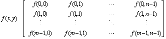(1)

Where, the row number is m-1 and the column number is n-1, which is indexed by j and i respectively. Note that in MATLAB^®, the matrix of digital image is counted from zero. If the position starts from 1, then they become m and n.

B. Basic properties of pixel

Each element in matrix at right hand of equation (1) is a function with specific location in a given coordinates system. The function f(x,y) contains specific meanings in digital image processing. RGB images are often used by human to store desired information in the form of colour. For a RGB colour image having m×n×3 sizes, each colour pixel is often resolved into three components, thus red green and blue (see Figure 10 ). The function f(x,y) in equation (1) is shown in the form of an arbitrary colour vector q(x,y) appeared in Figure 10 or Figure 3. Each colour component has individual gray-scale and is quantized in a digital image. Therefore the quantized scale is named as digital number. The colour vector q(x,y) can be expressed by equation (2). The colour sampling of observed objects such as lake, soil and vegetation shown in Figure 8 was implemented by the Image Tool™ in MATLAB^® in terms of this principle. The values of their R, G and B at the different locations (x,y) in Figure 8 are represented by Figure 11 (note that the unit of x,y depends on the one of scale used in x and y axis).

(2)

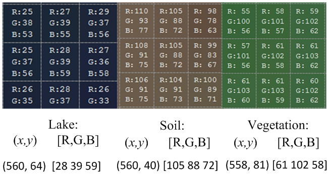
Figure 10. resolved color components of a size m×n×3 RGB image

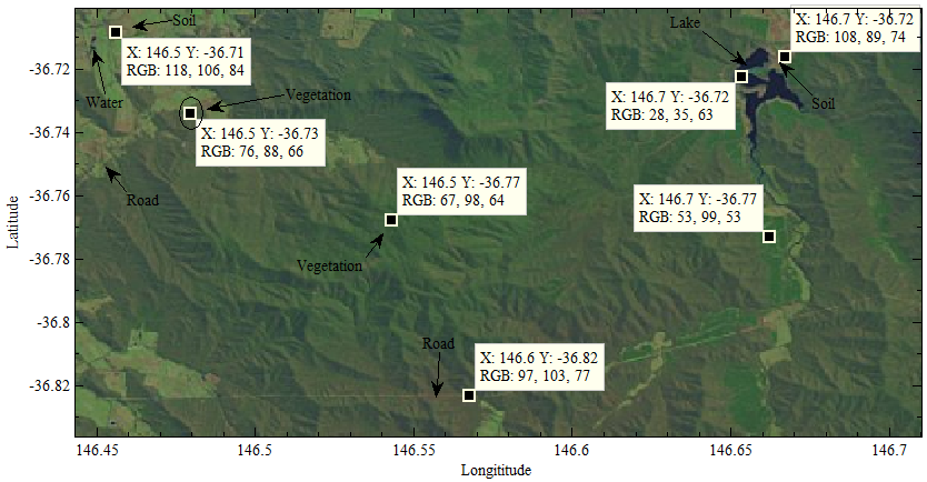
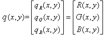
Figure 11. Color sampling of observed objects in the remote sensing imagery

Figure 12. schematic of algorithm for burning tendency test

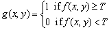
2.4. Burning Tendency Test

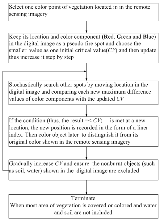
A. Algorithm of burning tendency

The algorithm of burning tendency test is developed from sampling diversely (see Figure 8 and Figure 11) in terms of spectral signature of substance (see Figure 2).

The general mathematical expression can be depicted by equation(3).

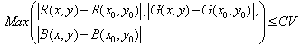(3)

In which, the CV is a critical value which is adjustable. The equation(3) is treated as criteria to assess whether each new spot (pixel) satisfies given CV during search for. The process of search is implemented from left to right and up and down (see Figure 12 ). The satisfied pixels are indexed and then coloured. The next search is performed by updating CV (from small to larger value).Updating CV is gradual to ensure typical objects like lake and soil are not coved by colour. The quick and precise algorithm of burning tendency test is illustrated in Figure 13.

B. An example of burning tendency test

A practical example is illustrated in Figure 14. In this example, the information for initial point of pixel (see Figure 8) is (x=129, y=117 or shown as x=146.5° y=-36.73°; R=76, G=88 and B=66). Note that the unit of pixel number was used rather than degree. The CV is set up as 10, then update CV step by step (see Table 1). The results are displayed in Figure 14 (1-6).

Table 1. bushfire tendency test in remote imagery and critical value State 1 2 3 4 5 6 Critical value (CV) 10 11 12 13 14 15

Of importance is that at the state 6, the most area of landscape are covered or coloured by red besides soil and lake. The most of coverage is vegetation. The covered area of vegetation is big enough to transfer the gathered information from it into DEM for modelling bushfire.

Figure 13. algorithm of burning tendency test

C. Possible physical interpretation for burning tendency test

Obviously, the classifying process may imply the following possible physical meanings on the basis of the technique of digital image processing and knowledge of combustion:

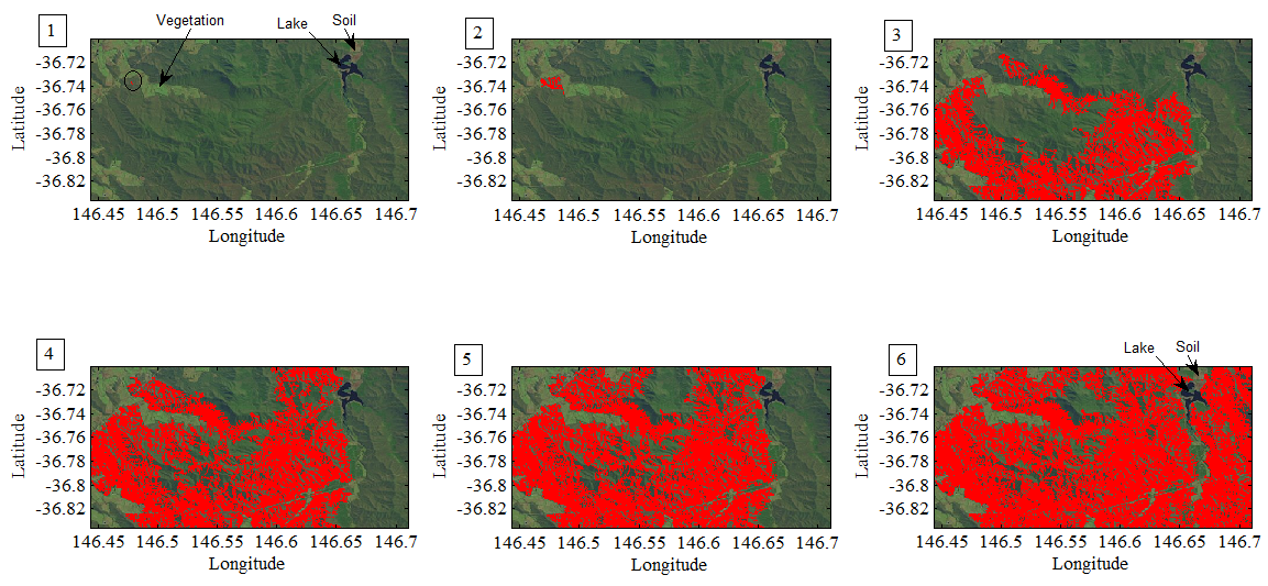Figure 14. burning tendency test in the remote sensing imagery

1. The point (x₀, y₀) is assumed as a spot where bushfire is initially ignited; the point (x, y) is hypothesized as a spot where bushfire possible spreads in the next burning zone. Consequently, the point (x, y) is a test point to seek for next burning spots stochastically after the initial point (x₀, y₀) (thus a burnt spot) is confirmed.

2. The point (x₀, y₀) is also stochastic and manually decided at any possible place where the vegetation distributed in the remote sensing image. This treatment may satisfy the real case if the bushfire weather is formed.

3. The area of vegetation is gradually classified and expended by increasing critical value step by step. Such a procedure implicitly represents the process of bushfire spread. The area of vegetation meets one critical value is burnt first and then named as a burning zone, the area of vegetation satisfying with the updated critical value is to be burnt at next step, which is defined as a smouldering zone.

Because each researching for new spots is from original spot after updating CV value, the spots whose CV values are less than update value are regarded as burnt areas or zone

Advantage and Disadvantage

Of importance for the burning tendency test is able to provide the information of distribution of vegetation at specific geographic location and the angle between the burning and smouldering zone with being unaware of the direction of bushfire spread.

However, the burning tendency test does not mean that the bushfire spread is to happen exactly following up the procedure provided by it.

The final result of bushfire spread shown in remote sensing imagery relies on initial position of vegetation and how the CV is chosen. The large CV may result in incorrect result. Therefore, what should be taken care of is to make sure

1. The initial location where vegetation is located.

2. The increase of CV cannot be too large for each step.

3. The lake and soil in the final result is not covered.

Furthermore, RGB-based burning tendency test is impossible to classify all substances like identifying substances using multispectral or hyperspectral imaging. However, in carrying out such a test, one feature such as spectral signature of substance was fully made use of. Therefore, this is different concept of identifying substances. The unique feature of in burning tendency test is that all classified objects (vegetation) are linearly indexed. The indexed objects are in position to be further handled and then accurately transferred into corresponding DEM. The multispectral or hyperspectral imaging does not have such functionality.

2.5. Classifying Burning and Smouldering Zone in a Remote sensing Imagery

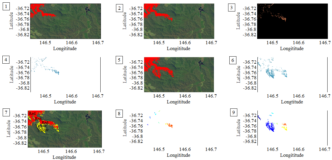
In bushfire tendency test, the extra area (thus the difference between new area and original area at one time interval) represents that the area of bushfire spread is enlarged from its original state with respect to elapsed time. If bushfire does not spread in the extra area yet, it can be named as smouldering zone.

The problem is that how to distinguish the smouldering zone (pixels) from previous zone (pixels). Directly distinguishing them using the existing linear indices is impossible. The technique that can be utilized is technology of digital image processing by means of the Image Tool™ in MATLAB^®.

However, processing a digital image associates with many concepts and techniques, it is impossible to detail them in this paper. A typical example of classifying burning and smouldering zone is illustrated as follows.

A. Some necessary steps in classifying burning and smouldering zone

There are three states of bushfire spread in Figure 15((1), (2) and (3)). They are generated by burning tendency test. The linear indices and pixels in the third state cover previous two states. Similarly, the second state covers first state.

Figure 15. illustrate the procedure of classifying burning and smouldering zone in the remote sensing imagery

Assume that the currently burning takes place at the second state and it approaches to the third state, similarly, for first state toward the second state. Very clear, some area (pixels) is not burnt yet and required to be distinguished. To do so, the first and second state is considered at first.

Step1: read two different images

Read the first and second state imagery using built-in function imread in MATLAB^®.

Step2: find difference of intensity

The difference of intensity between two images: f(x, y) and h(x, y) is expressed as

(4)

The g(x, y) is obtained by computing the difference of intensities between all pairs of corresponding pixels from imagery f and h. The built-in function: imabsdiff is used to obtain such difference of intensities between them. The result is shown in (3) of Figure 15. As seen, the new development of bushfire relative to the first state (1) is appeared. The background is black, which can be removed if want to see it clearly using the manner shown at the next step.

Step3: Inverse pixels

For a given digital image, it usually generates a pair of opposite relation in terms of difference of intensity for each pixel and designed criteria. The built-in function: imcomplement is able to generate an opposite effect. Applying it into the image in (3) yields the image in (4). Similar to the second and third state, the result is shown in (6).

Step 4: Save image

Save two full-object images in (4) and (6) into file separately for comparing them with their reduced results later using built-in function: imwrite.

At this stage, superficially it sounds that information kept by (2) and (5) have been lost because of changing their colours and cutting off other pixels. In fact, they are not; the rest objects are still able to be traced. The only problem is unsure what linear indices they are, but this problem is left here temperately. Therefore, the further treatment is required.

Step5: computes a global threshold (level)

Now focus on dealing with the smouldering zone between second and third state as assumed before. Before find it, the compliment of image in (6) (not shown) and similar to the image in (3) must be converted to be a binary image. In general, many fundamental operations in the digital processing happen in a binary image.

To do so, the approach is to find out a criteria based on the intensity of image. In fact, the thresholding is a simple process of comparison, one approach is that it is regarded as an extreme form of gray level quantization[21]. Suppose that a gray level image f(x,y) can take L possible gray levels 0,1,2,…,L-1. Define an integer threshold T, which lies in the gray-scale range ∈{0, 1, 2, L-1}. Then each pixel value in f(x,y) is compared to T. A binary decision is made by the comparison and appears in corresponding pixel of an output binary image g(x,y). The algorithm is that

A built-in function: graythresh provided by MATLAB^® uses Otsuian method, which is based on the normalized histogram. In this case, it is capable of gaining a global threshold using the values extracted from the blue or red band resolved from the original image. The function graythresh generates a normalized intensity value that lies in the range[0, 1].

Step6: conversion into a binary image

Up to this point, the compliment of image in (6), similar to the image in (3) is able to be converted into a binary image using the built-in function: im2bw.

Step7: find connected components of pixels in the binary image

Once the conversion of the compliment of image in (6) into a binary image is achieved, the connection of pixels for the third state can be dealt with using built-in function: bwconncomp. Then the generated value is inserted into other built-in function: regionprops. Those built-in functions provide several useful properties of image such as NumObjects and PixelIdxList. They supply information of number of connected objects and their corresponding linear indices. Eventually all indices for two smouldering zones thus the images in (4) and (6) can be picked up and confirmed.

Step8: show burning and smouldering zone using different colours in one image

Inserting linear indices of (2) and (6) into the same image assigning different colours such as red (burning zone) and yellow (smouldering zone) produces a new image in (7).

B. Display reduced burning and smouldering zone separately

However, from practical view, displaying all burning and smouldering zone separately requires a lot of memory in computer. The best way is to display selected area (e.g. the actual number of pixels in the region is larger than 80) like cases in (8) and (9), the colours ware added by built-in function: label2rgb for distinguishing objects in the same classified region. If compare cases in (8) and (9) with images in (4) and (6) respectively, the scales of objects in (8) and (9) are reduced. Such a treatment does not affect the quality of modelling because bushfire spread itself is a stochastic process. The small area is also burnt and covered. The objects in (8) and (9) are to be transferred into the corresponding DEM by using their discovered linear indices later.

As to detailed usage of built-in functions mentioned in this paper, refer to user’s manual of MATLAB^®.

2.6. Concept of DEM and Basic Properties

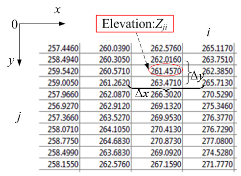Figure 16. data of DEM: elevation and corresponding grid interval

Mathematic Expression of DEM

DEM consists of tabulated data with fixed interval in horizontal and vertical direction (see Figure 16) can be visualized by three dimensions (e.g. Figure 21). As seen from Figure 21, DEM represents the bare ground surface without any objects like lakes, soils, vegetation and buildings. However, similar to digital image, DEM has several unique features.

a) At the plain level, in a coordinates system, mathematically speaking it is a matrix with fixed interval Δx and Δy along x and y axis.

b) In the vertical direction, each element in the matrix has corresponding elevation.

c) It has a direct relation with geometric feature of terrain.

Accordingly, to investigate the properties, the best manner is to consider it with the corresponding surface of terrain, which is to be introduced as follows.

Mathematic expression of terrain

To represent a section of curve of landscape on the earth, a general mathematic expression can be shown by equation(5).

(5)

Where is a continuous surface function of x, y in coordinates (z, x, y), z is elevation (see Figure 17 ).

If a boundary function y for boundary C in domain D is given, thus y=b(x), then the area of D is given by equation (6) in terms of Greenian theorem and the geometric properties of trapezoid(see Figure 17).

(6)

Where, the area of surface over D is

(7)

And the f _x² and f _y² is the second order derivative of a surface in x and y direction respectively.

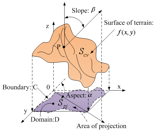Figure 17. mathematical expression of terrain

From equation(5), if , and c is an arbitrary constant, z is elevation. And then at the point P (see Figure 17), along its normal, it yields its gradient shown as

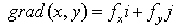(8)

Where, the i, j is the unit vector and the f _x ,f _y is the first order derivative of a surface function in x and y direction respectively.

The norm of equation (8) is named as slope, thus equation(9).

(9)

The slope represents the variety of elevation per unit length. Its corresponding angle is shown in the equation(10).

(10)

The range of slope angle is from −90° to 90°.

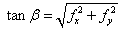
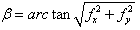
When f _x≠0, then the aspect (see Figure 17) is expressed as

(11)

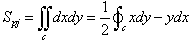
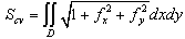
The aspect is the azimuth of the slope direction and its angle ranges from 0° to . In other manner, the aspect is also thought of as the direction of the biggest slope vector on the tangent plane projected onto the horizontal plane.

Defining the unit roughness R_k is based on the relation between the surface of terrain and DEM, which is defined as the ratio of the surface area S_cv to its projection onto the horizontal plane S_pj for the kth unit of surface area (see Figure 17).

(12)

The concept of slope, aspect and roughness is an important concept respectively. Many applications in development of GIS rely on them. Those geometric properties is impossible appeared in a remote sensing imagery for the same observed object at the same geographical location.

However, the analytical solutions to them are difficult to be obtained in practice; usually they can be resolved and applied in the form of numerical form. Nevertheless, they may be beyond the scale of discussion in this paper.

Figure 18. schematically illustrates the correlation between remote sensing imagery and corresponding DEM

2.7. Correlation between Digital Image and DEM

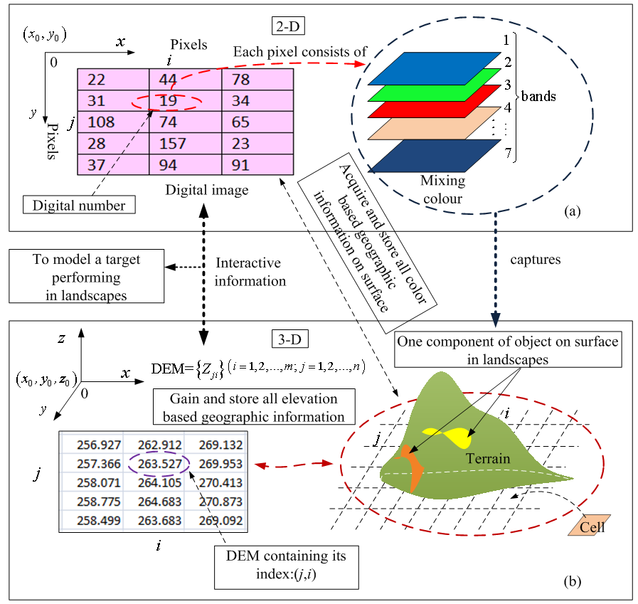
In the last sections, several vital concepts used in following fields were already introduced separately.

1) Digital image processing.

2) The principle of classifying vegetation in the remote sensing image to generate burning and smouldering zone.

3) Mathematically describing the surface of terrain.

4) Linking geomorphology to DEM.

At this stage, of importance is discuss how to connect two different coordinates system and accurately transfer collected data and information into other system and model specific case. Selecting the same location for both DEM and remote sensing imagery is the most important pre-condition for accurately establishing relationship between two and three-dimensional coordinates in those the same observed objects are located and transferring the interactive data.

The main unique features and functionalities associated correlation are summarized and illustrated in Figure 18.

Figure 18 shows that each paired index (j,i) in the satellite imagery (see Figure 18(a)) not only contains the digital number of each colour component stored in one pixel of the 2-D digital imagery but also links the corresponding elevation shown in the 3-D DEM (see Figure 18(b)). On the other hand, in the coordinates of DEM, a series of elevation Z thus{Z_ji},j=1,2,…,m, i=1,2,…,n, where m and n are integers, consists of DEM with m × n same size cells(thus, equivalent to pixels) . The subscript j and i are the same indices as the ones in the satellite imagery and denote the sequence of row and column respectively in a matrix, however, the paired index (j,i) can be merged into a linear index (see equation (13) ) in practice. In other words, the digital imagery has the same 2-D coordinates system as the one shown in DEM (refer to the coordinates: x-y and x-y-z in Figure 18). Mathematically speaking, for a satellite imagery and DEM having the same geographic location, a same size matrix exists in both of horizontal plains to describe the different physical properties (thus the digital number of colour and the elevation respectively) in the third dimension z. However, the digital number of colour is hidden in 2-D only.

2.8. Create Linear Indexing Using MATLAB^®

The technique of indexing is playing a vital role in developing GIS[22-26]. It is very useful to accurately link the same observed objects in different systems so as to effectively integrate and individually analyse the different physical properties appeared in the different systems. This process facilitates information and data exchange mutually.

MALTB^® is a matrix-based powerful package. If there is a matrix A with m×n size and subscripts are (j,i), the linear index is produced as follows.

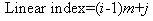(13)

Or

Use a built-in function sub2ind to generate a linear index for matrix A and then it is stored in the memory.

2.9. Conversion of Vector Point in the Coordinates of DEM

Figure 19. Vector point conversion in the coordinates of DEM

How to transfer the classified data into DEM was discussed previously by means of the technique of linear indexing. However, even if the procedure of accurately transferring data is achieved successfully, the implanted data in DEM from the remote sensing image is still ‘dead’. To model some ‘active’ behaviors in DEM, it relies on other technique named the vector point conversion in a given coordinates.

Assume that there is an arbitrary point A(x,y) in a grid-like coordinates system (see Figure 19 ). In fact, it can be exactly treated as a matrix with an arbitrary size. Also the origin point in the coordinates is assumed as O(x₀,y₀) and the row and column of the matrix is indexed by j and i respectively. The position of the vector point A(x,y) in the coordinates can be converted into the row and column indexed by j and i in the matrix by using equation(14).

(14)

Where, the sign[] is converting a fraction to be an integer. The d_x and d_y is a width of grid in x and y direction respectively.

Similarly, the index i and j must be into linear indices as equation(13).

As to the vector point conversion in DEM, several points must be taken care of:

1. This conversion only happens in a matrix-based DEM.

2. When the vector point A (x, y) is inserted into or created in m × n size DEM, it must be converted into a linear index using the algorithm mentioned in the section 2.8.

3. In practice, vector points could be many. They could represent spots of bushfire, water, smoke and any possible traced or observed objects. However, they must be converted into linear indices based on a given matrix (DEM) before they are accurately traced and further applied.

4. It should not be confused that the technique of vector point conversion in DEM generates the same linear indices as ones made in remote sensing imagery because both of them are based on the same dimension matrix, no matter which matrix is used.

5. Except whole data generated from the remote sensing imagery can be completely transferred into MED, so do partially selected data vice versa.

6. The difference in creating linear indices is that

1) In the case of remote sensing image, the linear indices are created based on the criteria of variation of colour (thus RGB).

2) In the case of DEM, the linear indices are created based on the criteria of variation of distance.

7. The linear indices are only a series of integers; they do not have any physical meanings for themselves. However, the indexed objects in different physical systems have individual own meaning. If each indexed objects are put together in one system by means of transferring selected linear indices, it certainly generates massive physical meanings.

8. Consider most modelling take place in DEM, therefore the technique of vector point conversion plays a vital important in modeling such as bushfire spread, smoke dispersion and even more.

2.10. A Simple Model for Determining Direction and Shape of Burning Spread

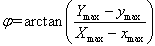
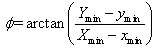
Determining the direction of the burning front is a hot spot in the bushfire investigation[27], some researchers used electric fans to generate wind in their laboratories and then determine the direction of burning front[28].

Determining Direction of Bushfire Spread in Terms of the Center of Mass

However, in modelling large scale bushfire in landscapes, the direction of burning front can be estimated by either meteorological measurement or connecting the corresponding mass centre located in the burning zone and the smouldering zone respectively. The latter was selected in this modelling. As to how to classify in the remote sensing imagery, refer to section 2.5.

The geographic location for the centre of mass of burning zone and smouldering can be decided by using a tool box: Image Tool™ in MATLAB^® as well (see point G and C in Figure 20).

The angle of bushfire spread can then be estimated by Equation(15).

(15)

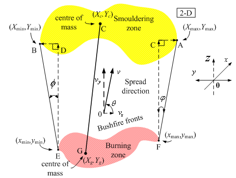Figure 20. Determine direction of burning front

Determining Laterally Expanding Angle and Displacement of Bushfire Spread

Although both mass centre (at the points: G and C) and the angle of bushfire spread can be confirmed, of importance in modelling is how to decide the direction and displacement of the burning front with respect to the increasing burning and smouldering area and the elapsed spread time. At this stage, the simple way is only to consider the lateral expanding of the bushfire remaining the original shape of burning front thus the fire front simultaneously spreads along the direction of lines: GC, FA and EB (see Figure 20). Therefore, it is not difficult to find out the minimum and maximum points in the burning and smouldering zone along the x direction. A pair of values: (x_min, y_min), (x_max, y_max) and (X_min, Y_min), (X_max, Y_max) illustrated in Figure 20 can be found by means of searching for the minimum and maximum values of position in the two zones. The sign v denotes constant average velocity of burning spread, which can be resolved into two components: v_x and v_y in the x and y direction respectively. As shown in Figure 20, two lateral expanding angles: φ and ϕ can be expressed by the equations (16)−(17):

(16)

(17)

Then both right and left side lateral displacement of the front with respect to the time of spread t can be approximately estimated by the equations:(18)−(19) while the bushfire spreads towards the smouldering zones:

(18)

(19)

2.11. Digital Elevation Model and Satellite Imagery Chosen for Bushfire Simulation

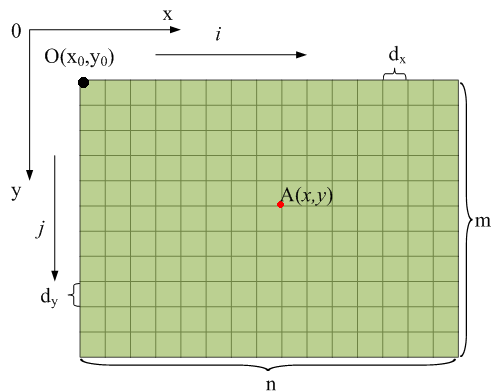
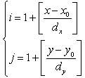
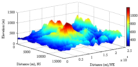
In practice, DEM is always located in a given physical coordinates. The unit often used to calculate is meter (see Figure 21) rather than geographic degree. Furthermore, the velocity is a vector. In order to position the movement of observed objects in landscapes, indicating the geographic orientation is necessary. The symbols NS and WE shown in Figure 21 are defined to denote the orientation of north-south and west-east respectively in a local Cartesian coordinates according to latitude and longitude indicated in Figure 8.

In this paper, the DEM chosen for bushfire simulation has the same geographic location (−36°70'10'' S, 146°44'30'' E; −36°83'60'' S, 146°71'00'' E) as the one of the satellite imagery (see Figure 8) captured by the satellite Landsat. In this area (Victoria, Australia), several large scale bushfires used to take place.

Figure 21. DEM is defined in meter

3. Results

3.1. Display Burning and Smouldering Zone in Digital Elevation Model

The geographic locations of burning (see Figure 22) and smouldering (see Figure 23) zones are transferred from those shown in (8) and (9) of Figure 15 respectively. This procedure is one important step for visualizing results and further approaches by means of data transfer.

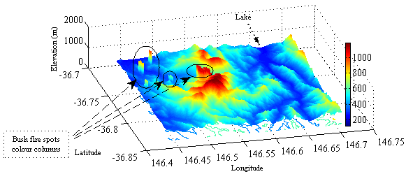Figure 22. Burning spots are located in burning zones

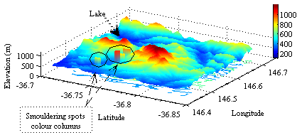Figure 23. Smouldering spots are located in smouldering zones

3.2. Bushfire Spread in Digital Elevation Model

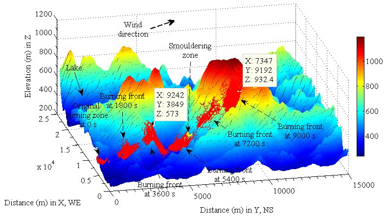
According to the proposed model (see section 2.10), the bushfire spread is assumed downwind and the constant average velocity is equal to . The result of modelling demonstrates this process in landscapes (see Figure 24). The detail is illustrated in Figure 25. In this application, the conversion between positions of bushfire spread and the local coordinates is required (see section 2.9) except for using the technique of linear indexing to transfer information from remote sensing imagery (see (7), (8) and (9) in Figure 15; Figure 22 and Figure 23).

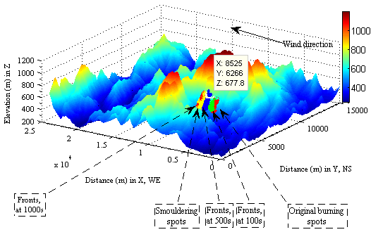Figure 24. Bushfire spreads from original spots to smouldering spots with average velocity ()

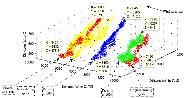Figure 25. Detailed bushfire spread with the constant average velocity

3.3. Display Information from DEM in Digital Imagery

In the last example, modeling bushfire spread in DEM was performed on basis of transferred data from remote sensing imagery and the technique of indexing and vector point conversion. Similarly, the result produced by modeling in DEM is also able to be displayed in the corresponding remote sensing imagery to verify the result.

Figure 26. modeling bushfire spread in DEM based on the geographical information and collected data transferred from digital imagery

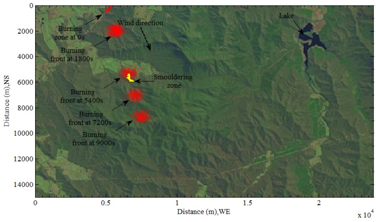Figure 27. Display selected information of modeling from DEM in the original digital imagery

The result shown in Figure 26 was implemented by a stochastic model. To reverse this process, what can do in MATLAB^® is that

Step1: read original remote sensing imagery (see Figure 8 ).

I= imread('Landscape.png'); % load image

Step2: design colour to distinguish object.

colour=[255; 0;0];% red: burning zone

Step3: resolve its three primary colour components.

R=I(:,:,1); % red component

G=I(:,:,2); % green component

B=I(:,:,3); % blue component

Step4: insert obtained linear indices thus ones generated from the modelling occurred in DEM into them assigning desired colour to them respectively.

R(Indices)= colour (1);

G(Indices)= colour (2);

B(Indices)= colour (3);

At this stage, each extracted colour component is indexed by linear indices and has the same colour: red.

Step 5: assign indexed red colour to the original remote sensing imagery.

I(:,:,1)=R;

I(:,:,2)=G;

I(:,:,3)=B;

Step 6: similarly, add smouldering zone into.

Step 7: Write modified original image with a new name into file.

imwrite(I,'fire_in_image.png','png');

Step 8: reread it and locate it in figure by adding scale.

Eventually, the original remote sensing imagery of landscape becomes one like Figure 27. Such approach not only enhances the effect of modelling but also easily verifies the result of modelling in new surroundings.

4. Discussion

As seen from (8) and (9) of Figure 15 and Figure 22−Figure 23, the data chain can be established within two different dimensional systems if the corresponding scale in two different coordinates is consistent. Through the data chain, the desired information is transferred from 2-D imagery into 3-D DEM. Of importance for modelling bushfire spread in landscapes is to know distribution vegetation. The process has been achieved by indexing the same observed objects during data transfer. It is obviously discovered that bushfire spread varies with slopes of terrain under the constant average velocity and the width is increased with the forward movement of bushfire front (see Figure 25).

On the other hand, most results generated in DEM can be reversely displayed in the remote sensing imagery (see Figure 26 and Figure 27 ). Above two example have proved how much important the linear indices are. Although they are generated in different manner, they have same integers due to the same size matrix they are used. They can be selectively transferred into other system to model some behaviour and display results. Furthermore, the some attributes of substances and objects can be altered relying on liner indexing.

5. Conclusions and Future Work

A. Summarize the current work

Several important and basic concepts and techniques used in modelling bushfire spread have been briefly reviewed and creatively proposed. The following targets in this paper have been achieved:

1. The useful information about the distribution of vegetation was extracted from the two-dimensional based remote sensing imagery to ensure bushfire occurs within bushes. The principle was also introduced descriptively. This is a pre-condition for modelling bushfire in the large scale landscapes.

2. The technique of indexing used to indicate the same observed object within two -coordinates system was explained in detail. This technique is very useful in temporal and spatial modelling.

3. The classified data were successfully transferred into the three-dimensional based DEM and displayed by means of the technique of indexing. It plays a vital role in transferring and visualizing data.

4. A technique of converting a vector point in a coordinates into a corresponding matrix was discussed. This is one of vital techniques for modelling bushfire spread in landscape using DEM.

5. A simple model used for determining direction of bushfire spread in terms of the measured centre of mass for both burning and smouldering zone was proposed. This is an ideal model only used for testing how to apply the transferred data into modelling bushfire spread in landscapes.

6. A demonstrated modelling bushfire spread in DEM was carried out. This practice is a foundation to further improve the proposed model of bushfire spread.

7. The selected information which gained and implemented in DEM has been displayed in the original remote sensing imagery to verify the results of modelling.

As seen, linear indices play an important role in indexing objects in different physical systems, modelling in another system (DEM) and reversely displaying results of modelling into the original system where desired data are collected and transferred from.

B. Future work

However, as mentioned at the beginning of this paper, more significant issues have been brought forth during this research and to be considered and carried out in the future study:

1. In order to apply transferred data into application, a simple case of bushfire spread in landscapes using DEM has been studied. This simple case indeed implies much potential, significant and various meaning. For DEM itself, a lot of geographic features hidden in it such as surface area, slope of terrain can be explored and applied. The slope is one of most important geographic parameters. It can be considered for calculating the surface area of burning on the basis of the plain area from the given satellite imagery.

2. To simplify the case supplied in the paper, the average velocity of bushfire spread was assumed as a constant. However, in reality, bushfire spread at surface is influenced by not only the distribution of vegetation in landscapes but also the features of terrain and meteorological factors. Therefore, the idea for estimating the real velocity of bushfire spread may be yielded from the one of local wind. A modified coefficient will be introduced into the real velocity of wind and then establish a comprehensive correlation between two different velocities may become quite necessary. The real velocity of wind may be estimated by using the geostrophic wind.

3. Naturally, bushfire spread and smoke spatial dispersion can be simultaneously modelled based on the technique of indexing and vector point conversion.

4. The corresponding mass and energy released from the burning bushes can be estimated on the basis of other physical models. The energy in this approach will be a real quantitative calculation by means of some valuable parameters from DEM, the theory of transport phenomena. Those approaches will be different from the concept of energy accounted for the principle of remote sensing in this paper.

ACKNOWLEDGMENTS

Author wants to offer special thanks to Professor Jing. X. Zhao at Shanghai Jiao Tong University for supplying desired data used in this research.