1. Introduction

The mapping of a road network and the determination of detailed road geometry is a task useful in many applications, i.e., verification and/or inspection of the geometrical characteristics of constructed roads[1],[2],[3]; mobile mapping[4],[5]; map matching and real-time mapping [6],[7]; consistency analysis of road elements and their influence on operating speed and traffic safety[8]; analysis of road geometry on driving conditions and visibility[9]; etc.

Road geometry is measured with the help of mobile mapping systems always employing vehicle-based GPS /GNSS receivers[6],[10],[11]. Additionally, the vehicles can be equipped with different monitoring sensors, such as CCD cameras[12],[13] and laser scanning systems[14],[15].

In this paper, the results are presented of a study about a mobile low-cost dual-DGPS mapping system for the fast tracing of the basic road design elements (horizontal plan, long section and cross sections). It is based on the use of GPS/GNSS technology and the requirements set by the guidelines of the Greek Ministry of Infrastructure, Transport and Networks (GMITN).

In order to formulate the principles and rules which govern the design of a road alignment, it is necessary to investigate the relation between the geometry of the road as a function of the vehicle velocity and the friction on the pavement.

A comparative study[16] of several road tracing regulations from Europe and the USA as well as of relevant research has led to the conclusion that there are several and essential differences in the selection of the permitted values of the friction coefficient, which is given by the following formula:

(1)

where:

f_R[-] = transverse friction component coefficient.

q[-] = transverse road inclination (cross-fall).

V[km/h] = vehicle velocity

R[m] = curve radius

These differences have, in term, decisive influence on the calculation of the minimum curve radii, the required visibility lengths, the minimum radii of convex and concave vertical curves, etc. in interdependence with the occasionally applicable design velocities.

In addition to the above, the determination of an adequate safety margin is always required in relation to the vehicle movement dynamics as most regulations do not define the theoretical basis according to which the permitted friction coefficient values are being proposed.

Concerning friction values, the “Safety Criterion III” (as included in the GMITN guidelines) was considered in this paper and is presented below:

Case 1: Good Road Design Quality

f_R – f_RA > 0,00

Case 2: Average Road Design Quality

-0,04 < f_R – f_RA < 0,00

Case 3: Bad Road Design Quality

f_R – f_RA < -0,04

where:

(2)

f_RA[-] = Design transverse friction component coefficient.

q_RA[-] = transverse road inclination (cross-fall) by the road design.

V₈₅[km/h] = operational vehicle velocity of the road design.

R_RA[m] = curve radius of the road design.

The comparison of the friction values in the above mentioned cases 1-3 can take place between the (f_RA) values of the design (or the prospective constructed) and the real continually updating values (f_R). These “real” values can come of a system which can provide the basic 3D geometry of the road and also the velocity of the vehicle. Such a system can be the low-cost GPS/GNSS system under consideration.

In order to verify the road geometry, classical surveying techniques can be used with accurate results. But this is an expensive and time-consuming task to utilize considering the hundreds kilometers of road that have to be surveyed. The problem becomes even more urgent when many kilometers of constructed roads have to be quickly inspected for geometrical safety or damage due to extreme natural phenomena (e.g., earthquakes, floods, landslides etc.).

To meet the above mentioned needs, a mobile low-cost dual-DGPS system was used. The system consists of a moving vehicle equipped with two GPS receivers placed on top of it on a special frame. Both these receivers were L1 GPS receivers of the same manufacturer and type and the distance between them was exactly equal to 3 m.

2. Description of the Experiment

In order to evaluate the system, classical geodetic measurements (using total station) were used in order to determine the as-built data of a newly constructed road segment. The experimental field was a recently completed approx. 0.5 km road at the outskirts of Thessaloniki being part of a service road of Egnatia Odos Highway (figure 1). The road has a width of 7 m, divided into two lanes each measuring 3.5 m wide. Three series of points were measured during the as built procedure: one at the left edge line, one at the centreline and one at the right edge line of the road respectively. The points were taken every 5 m, a distance which corresponds to a vehicle speed of approximately 18 km/h and 1-sec GPS acquisition rate. In this way, the slope along the road was determined and, accordingly, the cross-falls across the road were also computed.

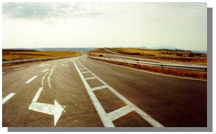Figure 1. The experimental field - a segment of a service road of Egnatia Odos highway, nearby Thessaloniki

The measurements by the mobile experimental system were carried out more than a year after the as-built measurements. The travel of the vehicle inside each lane gave GPS measurements of points close the centreline of the road (going and returning) from the left receiver as well as close to the right edge line (going) and the left edge line (returning) of the road from the right receiver respectively (figure 2).

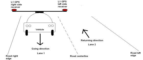Figure 2. The setup of the experiment

The GPS method used in this experiment was kinematic DGPS. Two base station receivers were operating at a distance from the road site. One of them was the Thessaloniki Continuous Reference GPS Station that started to operate at the facilities of the Laboratory of Geodesy & Geomatics in autumn 1999[17]. The other base station receiver was installed at a trigonometric point of the geodetic control network of the city of Thessaloniki. Raw data was collected every 1 sec and stored for about twenty minutes. After an initialization period, the vehicle travelled along the first lane of the road from one end to the other, and then travelled back along the other lane (figure 2). This procedure was repeated several times at different speeds, as following:

● two passings at 10-15 km/h (Datasets 1015A&B),

● two passings at 20-25 km/h (Datasets 2025A&B),

● two passings at 30-35 km/h (Datasets 3035A&B), and

● one passing at 50-60 km/h (Dataset 5060A).

The road length of the experiment was 425 m, from kilometer 9281.86 to 9706.86. Cross-sections were cut in this road segment every 5 m, thus providing 85 cross- sections to study.

3. Data Processing and Results

Upon completion of the field measurements, the computation of the co-ordinates of the points was done at the office by using the data of the two base station receivers and Kinematic DGPS software. Following the processing of data, it was found out that the accuracy obtained for the computation of the GPS points was ± 3 cm for most part of the road surveyed, regardless of the vehicle speed[5].

By using the known geometry (cross distance 3m and almost in the same level) of the system installation, first a logical filtering of the produced 3D coordinates of the dual GPS receiver system was performed. The point clouds which remained for every velocity and every passing were the data which can be used for the production of 7 different Digital Pavement Surface Models (DPSMs). Also, based on the measurements of the as-built procedure, the as-built road geometrical elements were reconstructed, a task that resulted into a unique horizontal plan, a unique long-section and the 85 cross sections mentioned above[2].

Some detailed drawings of the results of the above mentioned study are given in figures 3 - 5.

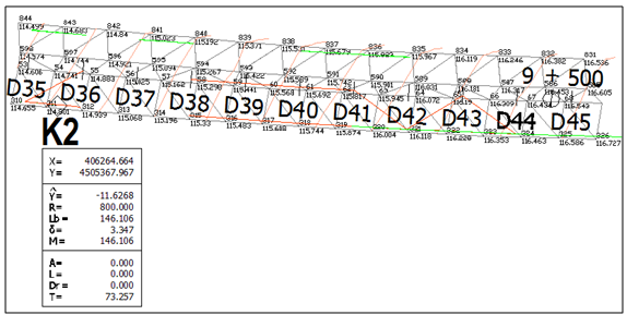Figure 3. Detail of the reconstructed road horizontal plan, DPSM by velocity 20-25 km/h, passing B

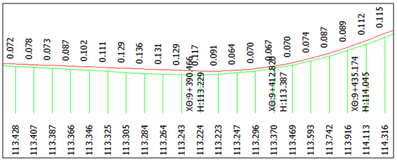Figure 4. Detail of the reconstructed road long section, DPSM by velocity 20-25 km/h, passing B

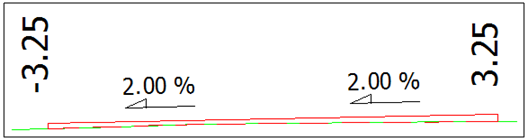Figure 5. Example of the reconstructed cross sections, DPSM by velocity 20-25 km/h, passing B

For the evaluation of the resulted data, Exponential Smoothing and Damped algorithms were used. Two sets of data were considered:

1. The height differences (DHsà DGPS heights for every pass minus as-built heights)

2. The differences between the DHs of every velocity-pass minus the DHs of the 10-15B km/h velocity pass, which has been chosen and used as “zero measurement” of the system in real measurements environment.

By using the above mentioned sets of data for every velocity and the exponential modelling theory, it becomes possible to re-construct and mathematically model the pavement long-section curves[18]. Also, to extract conclusions about the seasonality and the trends of the data and its residuals in different velocities. Furthermore, it could be possible to re-construct the two borderlines and to get conclusions about every cross-section.

In this paper, only the long-section evaluation is presented, making use only of the road-centreline data. But the same methodology can be applied in the same way also for the road-edges, providing the possibility to inspect the cross- sections too.

3.1. A Brief Report on Exponential Theory

The well-known formula for simple exponential smoothing is[19]:

(3)

If α is equal to 1 (one) then the previous observations are ignored entirely; if α is equal to 0 (zero), then the current observation is ignored entirely, and the smoothed value consists entirely of the previous smoothed value (which in turn is computed from the smoothed observation before it, and so on; thus all smoothed values will be equal to the initial smoothed value S₀). Values of α in-between will produce intermediate results.

In addition to simple exponential smoothing, more complex models have been developed to accommodate time series with seasonal and trend components that can be used for modelling the slope changes of the test pavement. Τhe two-way classification system has been used for the elaboration of the measurement data of the present paper. This system discusses the different models in terms of seasonality (none, additive, or multiplicative) and trend (none, linear, exponential, or damped). Specifically, the additive seasonality and the complex (linear & damped) trend components have been examined as the most adaptable for our case of observations.

3.1.1. Additive Seasonality Model

(4)

In this formula, S_t stands for the (simple) exponentially smoothed value of the series at time t, and I_t-p stands for the smoothed seasonal factor at time t minus p (where p is the length of the season). Thus, compared to simple exponential smoothing, the forecast is "enhanced" by adding the simple smoothed value by the predicted seasonal component. This seasonal component is derived analogous to the S_t value from simple exponential smoothing as:

(5)

3.2. Zero Dataset Selection

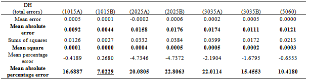
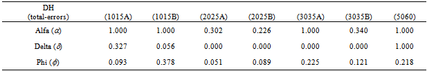
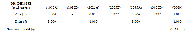
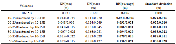
The simplicity of the method is based on well-known analysis techniques of geospatial data. Many times in spatial monitoring applications a dataset is used as the zero-dataset, thus setting a comparison level for the analysis of differences. This technique helps to avoid a complex simulation modelling of the vehicle oscillation, due to vibration of its mechanical parts when it operates.

The best fitting dataset after the implementation of exponential smoothing filters –containing seasonal, linear trend and damped trend components – was set as the operating moving vehicle model or zero-dataset.

Then, the remaining part of the height differences, which sums only the total estimated error of the 3D & low-cost mobile-mapping system was examined for every velocity pass (or dataset).

After the evaluation which appears in table 1, the best dataset to be used as the zero measurement can be estimated. Based on the quasi-Newton function[20],[21] and the well-known lack of fit indicators, Mean Squared Error (MSE) & Mean Absolute Percentage Error (MAPE)[22],[19], the 10-15B dataset was chosen as zero dataset, because it seems that its shape has the less deviation and it is the most independent of the moving vehicle statistical noise.

Tables 2 & 3 give the basic characteristics of the produced exponential models, which can be evaluated based on the following interpretation of indexes α, δ, γ and :

● If α is equal to zero (0), then the current observation is ignored entirely; if is equal to one (1) then the previous observations are entirely ignored.

● Seasonal parameter: if δ is zero (0), a constant unchanging seasonal component is used to generate the one-step-ahead forecasts; if the δ parameter is equal to one (1), then the seasonal component is modified at every step by the respective forecast error.

● Trend parameters: if the γ parameter is zero (0), the trend component is constant across all values of the time series; if the parameter is (1), then the trend component is modified from observation to observation by the respective forecast error. Parameter is a trend modification parameter, and affects how strongly changes in the trend will influence the estimates of the trend for subsequent forecasts, that is, how quickly the trend will be "damped" or increased.

It was observed that after the implementation of the zero-measurement:

● The dataset of 50-60 Km/h passing was not changed.

● The other exponential smoothing models generally became more dependent to historical (previous) data during the passing, which means a more reliable model fitting.

● The seasonal component almost disappeared or became a random noise.

● The trending component totally disappeared, except for the 50-60 Km/h dataset where it remained almost the same.

Table 4 gives the resulted total statistical verification data of the exponential smoothing processing for every velocity dataset in comparison with the same datasets after the implementation of zero-measurement, which means after the subtraction of 10-15B dataset.

Table 1. Height difference models evaluation by using Quasi-Newton method

Table 2. Basic characteristics of height difference models

Table 3. Basic characteristics of reduced (to 1015B velocity) height differences models

Table 4. Total statistical verification data of the exponential smoothing processing

In figure 6, the exponential smoothing results for 10-15B velocity pass is shown, which has been used as zero- measurement.

In figures 7 – 12, the velocity pass datasets per kilometre and also the optimum results of the exponential smoothing are given. Also, in comparison to figure 6, the respective results after the subtraction of zero dataset (10-15B velocity) from every other velocity pass (or dataset) are given.

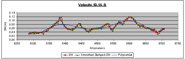Figure 6. Height differences per kilometre, their correspondent smoothed height differences and residuals for velocity passing 10-15B (km/h), which was used as zero-measurement

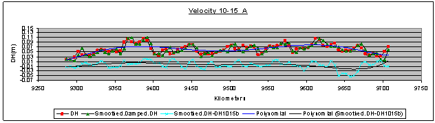Figure 7. Height differences per kilometre, their correspondent smoothed height differences and residuals for velocity passing 10-15A (km/h) and reduced velocity passing 10-15A (km/h) to 10-15B (km/h)

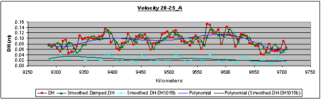Figure 8. Height differences per kilometre, their correspondent smoothed height differences and residuals for velocity passing 20-25A (km/h) and reduced velocity passing 20-25A (km/h) to 10-15B (km/h)

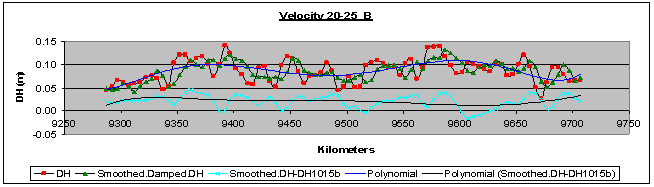Figure 9. Height differences per kilometer, their correspondent smoothed height differences and residuals for velocity passing 20-25B (km/h) and reduced velocity passing 20-25B (km/h) to 10-15B (km/h)

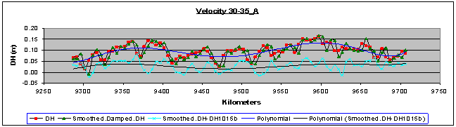Figure 10. Height differences per kilometre, their correspondent smoothed height differences and residuals for velocity passing 30-35A (km/h) and reduced velocity passing 30-35A (km/h) to 10-15B (km/h)

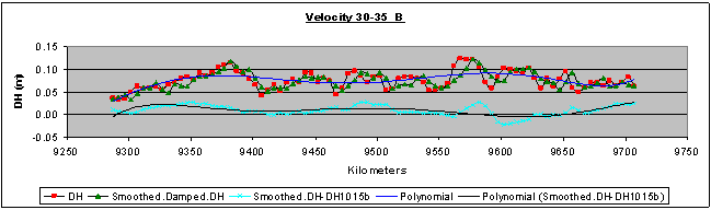Figure 11. Height differences per kilometre, their correspondent smoothed height differences and residuals for velocity passing 30-35B (km/h) and reduced velocity passing 30-35B (km/h) to 10-15B (km/h)

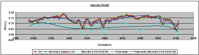Figure 12. Height differences per kilometre, their correspondent smoothed height differences and residuals for velocity passing 50-60 (km/h) and reduced velocity passing 50-60 (km/h) to 10-15B (km/h)

4. Results

It must be reminded that the key data used in the computations were the height differences between as built measurements (considered as known) and the corresponding GPS measurements in every velocity pass.

The results, shown in coral colour line and entitled “Smoothed.DH-DH1015b” in every figure from 7 to 12 are the remaining part of the total height differences, which are the sum of sedimentation or uplift plus the “no dynamic” and “dynamic” positioning errors of the tested road long-section in different velocities, after the removal of the zero dataset.

The zero dataset has been used to give a reference profile of the road long-section taking under consideration the specific mobile-mapping system and also the specific road segment and its surface micro-anomalies. The zero dataset includes the sum of sedimentation or uplift plus the “no dynamic” positioning errors of the tested specific road long-section in different velocities by using the specific mobile-mapping system (the same vehicle and the same instruments and installation)

So, this remaining part represents the “dynamic” positioning errors, the coral line being their profile. Also, the black line entitled “Polynomial (Smoothed.DH-DH1015b)” is a first attempt to model these dynamic positioning error profiles. The scope is to create a diachronic database for every road segment, which will be monitored by the specific mobile-mapping system and also to choose the optimum velocity to use in the practical application of the system.

In a similar way, it is possible to re-construct also the two borderlines and estimate conclusions about every cross- section. As a result, the reliability of the mobile- mapping procedure can be improved using more computational methods and not expensive instrumentation.

Finally, taking into account the “Safety Criterion III” and its classification as well as the above discussion, formulas (1) and (2) can now be used for the estimation of the as built road quality because the (f_RA) values of the design are known and the real continually updating values (f_R) can be computed by the system.

Consequently, the parameters of formulas (1) and (2) now read:

f_R = Observed transverse friction component coefficient (can be computed by the system).

f_RA = Design transverse friction component coefficient (known).

q = transverse road inclination (can be computed by the system).

q_RA = transverse road inclination (cross-fall) by the road design (known).

V[km/h] = vehicle velocity (observed).

V₈₅[km/h] = operational vehicle velocity of the road design (known).

R[m] = curve radius (can be computed by the system).

R_RA[m] = curve radius of the road design (known).

And, finally, the value of the comparison f_R – f_RA of f_R (computed by the system) and f_RA (known) can be used for the evaluation of the quality of the as built road or the current situation of the road, according to the “Safety Criterion III”, as stated in paragraph 1 (good, average, bad).

5. General Conclusions - Discussion

In this paper, the results of an investigation about a mobile low-cost dual-DGPS system for the fast tracing of the basic road design elements were presented.

The procedure has the aim to work as a tool for decision making concerning the operation and the maintenance of roads and is based on repeated measurements with the same system-components (same vehicle and sensors). This concept will include only the three basic road design drawings, which are horizontal plan, long section and cross sections and not the detection of local pavement anomalies.

Concerning the results of field data and statistical analysis, following remarks can be done:

● In all vehicle passing cases, the average height differences were negative, a very logical fact, because the experiments were carried out more than one year after the as-built measurements and the operation of the road. Thus, settlements were expected to be observed as this road segment is part of a road network in an industrial area hosting the traffic of many heavy vehicles.

● The use of the 10-15B Km/h pass as “zero-measurement” gave the opportunity to extract some very useful conclusions. This pass was chosen based on quasi-Newton method, where the main lack of fit indicator (mean absolute percentage error) delivered the minimum value (7.0229).

● The reduction of 10-15B km/h pass from the remaining passes removed from the height differences (DHs) the total error of the procedure, the real settlements of the pavement and a part(no dynamic) of the error of DGPS measurements and processing. The remaining part gave the unknown noise of the mobile system GPS frame – vehicle (dynamic part).

Also, it became obvious that, generally, as the velocities increased, the reliability of the system decreased. It was concluded that a velocity of 20-30 km/h could be the optimum operational velocity of the mobile system.

It is certain that a critical factor is the cost of the system. Today, more integrated systems can be used providing reliable results related to road characteristics documentation. But the simplicity and the low cost of the proposed methodology may give the opportunity to equip a significant number of available maintenance vehicles with L1 GPS receivers for the same cost of a single mobile GPS/INS/ TLS/camera system.

The procedure and also the algorithms of this decision making tool can be improved in the framework of the classification of the pavement not only based on its geometric characteristics, but also by tracing the quality of its surface with support from high-speed digital cameras. This can help considerably to the updating and redefinition of the pavement friction coefficients of vehicles safety specifications based on the real operative conditions of the road.