-
Paper Information
- Next Paper
- Previous Paper
- Paper Submission
-
Journal Information
- About This Journal
- Editorial Board
- Current Issue
- Archive
- Author Guidelines
- Contact Us
American Journal of Geographic Information System
p-ISSN: 2163-1131 e-ISSN: 2163-114X
2012; 1(3): 39-48
doi: 10.5923/j.ajgis.20120103.02
Modeling Bushfire Spread Based on Digital Elevation Model and Satellite Imagery: Estimate Burning Velocity and Area
 Abstract
 Reference
 Full-Text PDF
 Full-Text HTML
Carl Y. H. Jiang
Centre for Intelligent Systems Research, Deakin University, Victoria, 3216, Australia
Correspondence to: Carl Y. H. Jiang , Centre for Intelligent Systems Research, Deakin University, Victoria, 3216, Australia.
| Email: |  |
Copyright © 2012 Scientific & Academic Publishing. All Rights Reserved.
Several novel concepts and manners in modelling bushfire are introduced and defined on the basis of interdisciplinary knowledge. The velocities of bushfire spread are estimated by integrating the burning delay coefficient with the local geostrophic wind. The burning delay coefficient is a comprehensive factor consisting of a series of different properties existing in and varying with the process of fire spread. The grouped model used to assess the direction of burning zone and determine geographic location is proposed and applied. The distribution of burning spread in each burning zone is stochastic and the illustrated instances of burning zone spread are provided. The surface area of burning is also considered by means of the known size of pixel in the satellite imagery and individual slope extracted from the features of digital elevation model. The results of simulation are quite consistent with the real situation of bushfire in comparison with the scenario of bushfire captured by the satellite imagery.
Keywords: Bushfires Simulation, Satellite Imagery, Digital Elevation Model, Burning Delay Coefficient, Burning Surface Area, Bushfire Spread Velocity
Cite this paper: Carl Y. H. Jiang , "Modeling Bushfire Spread Based on Digital Elevation Model and Satellite Imagery: Estimate Burning Velocity and Area", American Journal of Geographic Information System, Vol. 1 No. 3, 2012, pp. 39-48. doi: 10.5923/j.ajgis.20120103.02.
Article Outline
1. Introduction
- Bushfire is a natural disaster that not only destroys forest, settlements, and life due to lack of necessary warning but also pollutes natural environment. Therefore studying how bushfires spread in landscape has been a worldwide hot spot. In reality, the fast-moving bushfire, as an important information, has seriously been attracted and studied by fire fighters and risk managers[1-2]. In the field of theoretic study, some researchers have proposed a few models by means of some experiments to simulate fire behaviour[1-2]. The relation between fire spread and speed of wind has already noticed and investigated by Beer[3-4] for a few years. However, the most of their researches were restricted within experimental scale. Therefore some parameters describing bushfire spread in landscape such as velocity and area of burning spread were impossible to be estimated by means of experiments. Very obvious, the experiment-based theoretic modelling has a prominent drawback; thence the results yielded from such modelling fail to represent a large scale bushfire in the landscape. In order to accurately and effectively model and forecast bushfire spread in large scale landscape, a novel method of integrating DEM (digital elevation model) with remote sensing imagery is to be introduced in this paper. However, it is necessary to outline some features of remote sensing imagery, DEM and some relevant issues as a primary knowledge so as to understand the reason why to carry out the approaches shown in the following sections in this paper.Features of Remote Sensing Imagery and DEMThe unique approach demonstrated in the paper is based on the interactive information extracted from DEM of landscapes and the corresponding remote sensing imagery respectively. Both DEM and remote sensing imagery have individual features and drawbacks.A. Remote sensing imagery:The advantages of it are able to provide1. The distribution of vegetation and other information such as lake and soil.2. The area of unit pixel which is equivalent to the real scale area at ground if the geographic location of it is the same as that of DEM.3. And so on.The drawbacks of it fail 1. To show and abstract three-dimensional information of geometric features of terrain such as slope.2. To model the movement of objects in landscape.B. DEM:The advantages of it are able to1. Extract geometric features of terrain such as slope, roughness and so on.2. Perform or model most of natural phenomena such as natural disaster and other behaviours in landscape.The main drawback of it 1. Fails to supply useful information such as distribution of vegetation on the surface of terrain.Above individual features of them point out a fact that modelling cannot be performed purely relying on one-side information.Data Transfer between Remote Sensing Imagery and DEMHowever, in practice, the existing drawbacks can be overcome by mutually transferring useful information and data. Thus, the information owned by the remote sensing imagery can be transferred into DEM by means of indexing technology. This process happens within two different coordinates system, thus the coordinates is set up in the remote sensing imagery and DEM respectively.Each coordinates consists of the same dimension matrix. However, the elements in the different matrix represent different physical properties. For instance, the elements in the matrix of the remote sensing imagery invisibly contain gray level of colour components (Red, Green and Blue) and the information hidden in the remote sensing imagery can be extracted by the technique of digital image processing. Nevertheless, it is beyond the range of discussion in this paper. On the other hand, as mentioned previously the elements in the matrix of DEM have other geometric properties besides elevation. The concept of slope is the most important parameter, which links two different areas in different aspect. On the one hand, if the area of terrain is dealt with numerically, in the real scale, it connects the unit surface area and the unit area located at horizontal level; on the other hand, it potentially connects such relationship hidden in the digital imagery while it was formed by the satellite. Discovering geometric properties relies on the techniques used in geography; such an issue is also beyond the scope of the research in this paper.However, of importance is that the information shown by remote sensing imagery must be accurately transferred into DEM by means of the technique of indexing. So-called technique of indexing is a process of accurately dealing with the collected data shown by a matrix. All elements listed in the matrix and represent different physical properties are indexed by a series of paired indices of column and row. When the specific performance is carried out, for instance, classifying the distribution of vegetation captured and stored in the remote sensing imagery, the paired indices of column and row are merged into a series of linear indices and then stored into the memory of computer. In fact, this process is a liner conversion from two-dimensional indexing to one- dimensional indexing. Finally, those data containing original information such as the geographical location and distribution of vegetation are visualized in the corresponding DEM. Again, DEM must have the same geographic location and dimension of matrix as those the remote sensing imagery has. Otherwise, modelling based on such an approach is impossible to perform correctly.Modelling in DEMOnce collected data from remote sensing imagery have been implanted into DEM, modelling can be carried by utilizing the geometric features of DEM. However, gaining a few parameters such as the surface area of terrain still depends on the information stored in the remote sensing imagery.In addition to, in this research, some parameters such as a velocity of bushfire spread ,which can be confirmed by making use of the knowledge of meteorology.In modelling specific case, for instance, the positions of moving objects in landscape, their positions in the coordinates of DEM must be calculated in terms of the specific principles of science and engineering. Meanwhile, the behaviours must simultaneously be indexed and then can be displayed. This process could be complex depending the case is to be modelled.No matter how to model a case in the landscape, the technique of indexing plays significant role in accurately tracing the motion of objects and effectively displaying the physical and physiochemical properties of observed object.Objectives and Scope of ResearchHowever, bushfire spread is a very complicated process. It requires multidisciplinary knowledge to quantitatively calculate and analyses its spread. Typically, for instance, the bushfire spread is accompanying with mass and heat transfer. It relies on a few important parameters such as temperature, area and velocity and so on to calculate them.Directly obtaining the values of those parameters by means of measurement is impossible. The effective method to obtain them is by means of an indirect manner which is to be introduced as follows. In this paper, the attention is restricted to investigate velocity and area involved in the bushfire spread and the modelling starts from the step at which the classified data of distribution of vegetation have been implanted into DEM.Therefore, the main aims in this paper are to explore 1. How to estimate the velocity of bushfire spread making use of the natural phenomenon - the velocity of geostrophic Wind.2. How to establish relationship between velocity of bushfire spread and that of geostrophic wind.3. What the potential geometric relationship between remote sensing imagery and DEM.4. How to estimate the unknown surface area of terrain shown in DEM integrating with the corresponding remote sensing imagery.5. How to model and estimate the velocity of bushfire spread using DEM.Eventually, the results obtained from simulation are to be compared with the real historical situation of bushfire spread acquired by satellite imageries at the same geographical location so as to analyses the quality of modelling and seek for possible resolutions to improve potential problems in the future research.
2. Methodology
2.1. Velocity of Burning Spread
- As mentioned above, the velocity of burning spread is a most important parameter in forecasting how fast the bushfire spreads, but it is very difficult for researchers to directly measure and estimate it based on traditional manners. The most convenient and effective manner being proposed in this paper is to establish relationship between the velocity of burning spread and that of local wind. As well known, in the burning zone, the local wind is composed of the geostrophic wind and the thermal wind. The former is a natural phenomenon owing to the rotation of the earth; the latter is caused by the heat free convection. However it is difficult to distinguish two different forms of wind in both analysis of theory and real measurement. In order to resolve such a difficulty, two important concepts namely the velocity of geostrophic wind and the burning delay coefficient are to be introduced as follows.
2.1.1. Velocity of Geostrophic Wind
- The geostrophic wind[5] is caused by the pressure gradient of atmospheric air and deflecting force due to the earth’s rotation.As shown in Figure 1, the actual wind at the surface of ground is determined by three forces: P, F and D respectively. The angle ξ approaches zero at the upper layer of atmospheric layer, usually ξ ≈25°−35° at the lower layer. The velocity of geostrophic wind Vgeo is calculated by using the following equation (1):
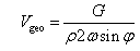 | (1) |
 = 1.166 kg m-3 at 30 °C, φ = −36.75°and calculated by the equation(1). Very obvious, the result shown in Figure 2 is a pure distribution of the actual velocity geostrophic wind without being affected by other factors. Nevertheless it plays a vital role in the calculation of following modelling.
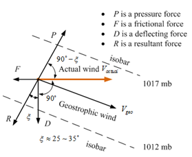 | Figure 1. Geostrophic wind at the surface of ground |
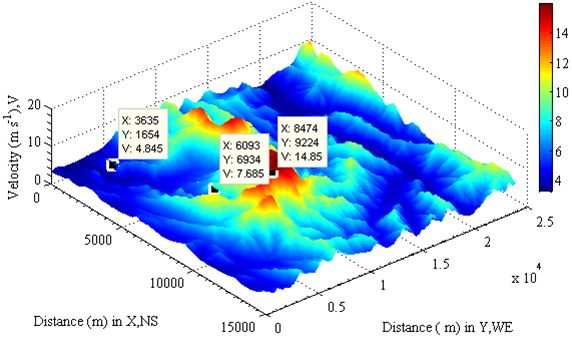 | Figure 2. Variation of geostrophic wind velocity with elevation per 100 meter is shown in DEM |
2.1.2. Burning Delay Coefficient
- Although the wind is able to accelerate the velocity of burning fronts, the velocity of wind does not equal that of burning fronts. Except for the factor of local wind (thus geostrophic wind and thermal wind), the type of vegetation is other main factor affecting velocity of fronts spread. In order to get a reasonable resolution, assume that the velocity of burning fronts Vb,k has the following relation with the real velocity of wind Vgeo,k at a local burning spot k.
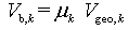 | (2) |
2.2. Define Geographic Location of Spread
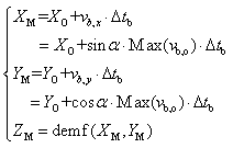
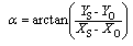
2.2.1. Position of Mass of Centre
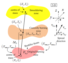 | Figure 3. Schematic presentation of bushfire spread in landscapes and definitions |
 | (3) |
 | (4) |
2.2.2. Position of Stochastic Burning Spots
- Due to uneven distribution of velocities of spread in the burning zone, a set of arbitrary burning points (Xb,c,Yb,c) having an arbitrary velocity of spread is used to position stochastic burning spots in the currently burning zone and in which, the subscript b and c denotes burning spots in the currently burning zone respectively. The positions of stochastic burning spots in it are determined by the equation (5).
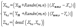 | (5) |
2.3. Define the Unit Surface Area of Spread
2.3.1. Roughness and Surface Area
- To calculate burning surface area, in this paper, of importance is how to determine the unit surface area of the terrain with respect to one unit area of pixel locating in a matrix of digital imagery. Hence, this approach is to establish the relationship amongst the geometric parameters: the surface area of terrain, its projection area, the slope between them (the slope is extracted from DEM) and the real scale area of terrain represented by each pixel in the remote sensing imagery. The basic principle is introduced as follows.First of all, the concept of the geographic roughness is required to be reviewed and developed. There are several definitions for the geographic roughness. However, in this paper, the roughness RE is defined as the ratio of the surface area and its projection onto the horizontal plane[6]. Its mathematical expression is shown in the equation (6) (see Figure 4(a) and (b)). Where, the subscript E is the domain of horizontal plain into which the sum of cell surface of terrain is projected, the subscript g denotes the sequence number of pixel within the domain E ; it is often a linear index in practice. The term Scv,g and Spj,g denotes the arbitrary cell surface area at the curve surface of terrain and the corresponding projected surface area on the ground (indicated by the subscript cv and pj) respectively. The more explanation about Scv,g and Spj,g is at the section 2.3.3. The symbol: fx2 and fy2 is the second derivatives of a continuous surface function f(x, y) in x and y direction respectively within domain E[7-8]. The L denotes the function of the corresponding boundary of domain E. The more detailed illustration of the relation between Scv,g and Spj,g and their projections is shown in Figure 4(b).
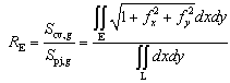 | (6) |
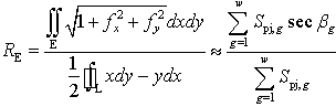 | (7) |
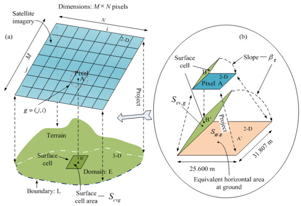 | Figure 4. Correlation between the area of cell surface on terrain and that recorded as one pixel in the corresponding satellite imagery |
2.3.2. Real Scale Area Represented by One Pixel and Surface Area
- In this paper, the dimension of the selected remote imagery in Figure 5 consists of 933 × 472 pixels whose size of each pixel is same; the corresponding DEM with real scale is shown in Figure 6. Therefore, the size of one pixel in Figure 5 thus the Spj,g is equivalent to 25.600 m ×31.807 m in a horizontal plain at the surface of the earth (see Figure 4(b)).
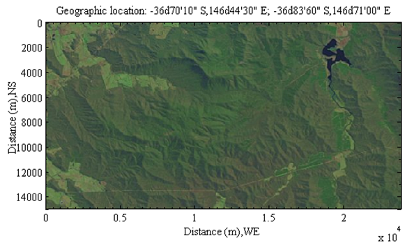 | Figure 5. Satellite imagery corresponds to the selected DEM |
2.3.3. Indexing Area and Pixel
- Although the values of both Scv,g and Spj,g can be shown in two separate coordinates located in the digital imagery and DEM respectively, at two dimensional level of each coordinates, the location of the same observed object that owns Scv,g and Spj,g can be determined by two same dimensional matrices established in two different coordinates (thus one in the given digital imagery[13-14] and another in the corresponding DEM). Accordingly, the Scv,g and Spj,g are also correlated and indexed by a set of linear indices {g} , where g= (j,i), the value of j and i is the sequence number of row and column respectively in a matrix of each coordinates see Figure 4(a)).In this case, the dimension of both matrices is 933 × 472.
3. Results
3.1. Local Burning Velocity Affected by Geostrophic Wind
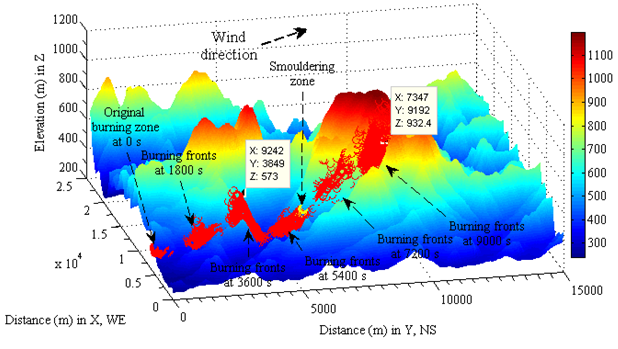
3.1.1. Positions of Fronts Spread
 | Figure 6. Bushfires stochastically spread downwind with constant burning delay coefficient and velocity of local geostrophic wind |
3.1.2. Velocities of Spread in Burning Zone
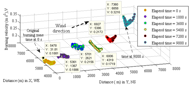 | Figure 7. Velocities of burning spots in different burning zones |
3.1.3. Fronts Spread with Updating Velocity
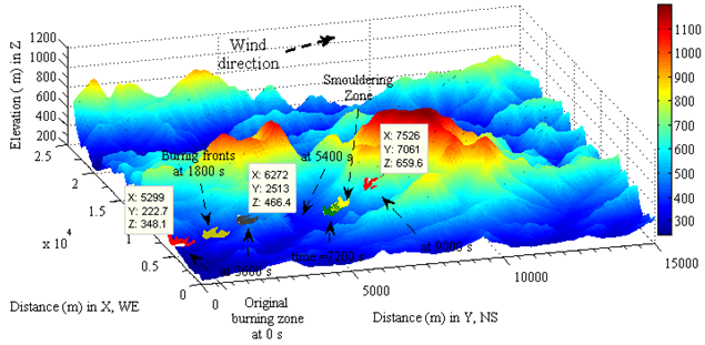
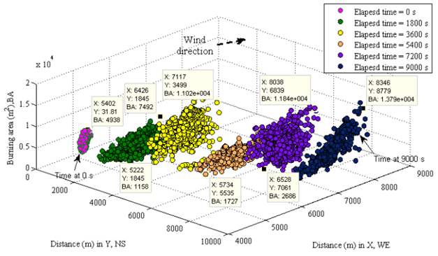
- In this case, the velocity of burning zone spread is a variable, thus calculated by the previous maximum velocity of geostrophic wind multiplying a burning delay coefficient (μ = 0.04) at different time interval. The mass centre for the original burning and smouldering zone is Xo= 5222.8 m, Yo= 294.1 m, Zo= 340.7 m and Xs=6690.0 m, Ys=5715.0 m, Zs=462.4 m respectively; the dimension of matrix for determining stochastic distribution of burning spots in x and y direction is m=1, n=1000. The result calculated by equations (2) − (5) is shown in Figure 8. The velocities in the burning zone are also influenced by both local geostrophic wind and distribution of vegetation, thus stochastic distribution in each burning zone.
 | Figure 8. Locations of bushfire spread influenced by variation of local geostrophic wind with constant burning delay coefficient |
3.1.4. Velocities of Mass Centre of Burning Zone
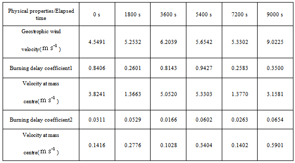
- However, the average velocity of burning spread may be concerned. To handle it, studying variation of mass centre of burning zone could be useful. In order to illustrate how the burning delay coefficient affects the velocity of burning zone and how much they correlate with corresponding velocity of geostrophic wind, a set of data is designed in Table 1. Two groups of burning delay coefficients are random numbers between zero and one and represent different properties at the surface, which have been mentioned above.Figure 9 based on Table 1 illustrates local the velocity of geostrophic wind varies with elevation. The burning delay coefficient is one of main factors influencing upon the velocity of fire spread, however, in general, the velocity of fire spread ascends uphill if vegetation exists and descends downhill.
 | Figure 9. Bushfire spread centre of mass at different time interval |
|
3.2. Local Burning Area
- The Figure 10 displays the surface area of instantaneous burning responding to Figure 8. Each burning area in a specific burning zone is different; however, of concern is the sum of those areas. The sum of burning area in one burning zone is valuable in estimating amount of pollutant such as smoke and released energy.
 | Figure 10. Instantaneous burning surface area of vegetation with respect to time interval |
4. Discussion
- The most effective manner to analyses results from modelling larger scale bushfire is comparing them with the information acquired by satellite imagery. Due to the limit of information supplied by satellite imagery in comparison with the three-dimensional based modelling; the discussion is only focusing on the discovered information from the satellite imagery.
4.1. Satellite Images of a Large Scale Bushfire
- In order to compare the results of simulation with the real situation, a group of satellite images acquired a large scale bushfire spread happened at the similar geographic location in Victoria, Australia are supplied in Figure 11.Where, the following information for Figure 11 is supplied by environmental system & services[15] as well.
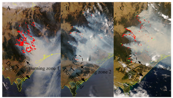 | Figure 11. December 2006 Victorian bushfire satellite images, Australia[1] |
4.2. Comparing Results of Modeling with Satellite Images of Bushfire
- According to the information of bushfire gained from the satellite imagery at the same geographic location, the result of modelling is almost consistent with the scenario in reality by comparison.
4.2.1. Similar Points
- 1. Local velocities in each burning zone depend on the magnitude and direction of geostrophic wind at different spots. Refer to the area and direction of smoke shown in Figure 11 and the results in Figure 6−Figure 8 whose direction was decided by the angle between mass centre in smouldering and burning zone.2. The magnitude of geostrophic wind is increased with the elevation. Therefore the burning velocities uphill is always larger than ones downhill, the burning velocities vary with change of geographic location. Refer to the intensity of uphill burning (imagery A) vs. the one of downhill burning (imagery B) with the same wind direction in Figure 11 and results in Figure 6−Figure 8.3. The bushfire spread of each burning zone is stochastically distributed. In reality, there may be many burning zones can be discovered from the real situation of the imagery A, B and C shown in Figure 11. The original burning zone was selected stochastically.4. The bushfire spread in each burning zone is stochastically distributed.The bushfire spread in each burning zone enlarges stochastically. Refer to burning zone1-3 in the imagery A-C in Figure 11.Therefore the assumption in modelling is consistent with the facts.
4.2.2. Different Points
- 1. Velocities of spreadThe velocities of spread in the reality may be much slower than one assumed in the modelling. The burning delay coefficient could be at the range between 10-3 and 10-4 rather than 10-2 which was assumed in modelling. Refer to the variation of location of burning spots in the burning zone 1 to 3 shown in Figure 11 with the elapsed time. This is the main difference comparing them with the result generated by modelling.2. Shape of spreadThis difference is caused by different distribution of vegetation and the features of terrain; however this is not important difference.
4.3. Advantages and Difficulties in Modeling
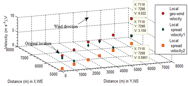
- Compare with two-dimensional based remote sensing satellite imagery of bushfire in forecasting bushfire spread and estimating amount of released energy and pollutant, the two and three dimension (thus 2-D landscape satellite imagery and 3-D DEM) based modelling has a series of distinguished advantages. The former passively traces the fire spread, the advantages of the later are unique, which are capable of: 1. Tracing the bushfire spread according to the given information about distribution of vegetation and measured direction of wind;2. Estimating burning area, this approach has been achieved and shown in Figure 10;3. Estimating Amount of released energy (which will be performed in the future research);4. Assessing the possible consumed time for bushfire spread from one location to another;5. And so on.However, the most difficult is to assess effective burning delay coefficient. In modelling, owing to selecting different values for velocity of spread remaining the same burning delay coefficient, it resulted in different result. For instance, the results shown in Figure 6 and Figure 8 are much different. The stochastic locations in Figure 8 was assessed by using pervious maximum velocity of local wind in each updated burning zone, however the one in figures 6 was calculated using the maximum velocity of local wind in the original burning zone thus the one at time = 0 second. The rough error of the direct distance is 2092 meters in 9000 seconds later, thus the error in assessing velocity of spread is equivalent to 0.8 km h-1.
4.4. Suggestion for Improving Quality of Modeling
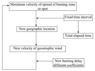
- Directly measuring burning delay coefficient is impossible. However, in order to accurately assess the velocity of spread, based on the approaches in shown in Figure 6, Figure 8 and Figure 9, the velocity of spread can be frequently updated by assigning different burning delay coefficient. The algorithm is shown in Figure 12. When the bushfire spread is moving forward, the burning delay coefficient simultaneously varies with the variation of the location. As mentioned previously, at new location, a lot of new comprehensive factors are represented by a new burning delay coefficient. In modelling is simply to assign a new value of the burning delay coefficient to the velocity of local geostrophic wind. The elapsed time is continuously accumulated. According to this algorithm, forecasting bushfire spread could be possible.
 | Figure 12. Suggested manner of improving accuracy in assessing velocity of spread |
5. Conclusions
- The approaches using DEM to seeking two important parameters: velocity and area and forecasting bushfire spread in landscape in this paper were based on the data which have already been transferred from the corresponding remote sensing imagery.In order to find out the effective and accurate methods in modelling large scale bushfire in landscapes, the following new concepts and manners have been proposed and achieved.1. The velocity of bushfire spread is yielded by integrating velocity of geostrophic wind with burning delay coefficient. This approach has overcome one of the difficulties which many researchers in the world have endeavoured to resolve it for many decades.When the bushfire spread, the thermal wind is another type of wind, which is caused by local heat convection. Although it plays certain role in accelerating the velocity of bushfire spread, its direction usually is towards the vertical because the driven force of heat convection is temperature gradient. The temperature at ground is always higher than the one in sky especially when bushfire takes place. Furthermore, the magnitude of thermal wind is much smaller than that of velocity of geostrophic wind. That is the reason why the velocity of geostrophic wind was chosen in this research. On the other hand, the local effect of thermal wind has already been considered in the burning delay coefficient. 2. The velocity of geostrophic wind is easily to be calculated and confirmed no matter how the bushfire spreads because the geostrophic wind is a natural phenomenon caused by the self-rotation of the earth. Once the velocity of geostrophic wind is treated as a criteria velocity, applying an adjustable a burning delay coefficient to it, effectively estimating the velocity of bushfire spread is much simplified. The process of bushfire spread can be forecasted rather than passively being tracked by means of the monitoring of the time limited satellite. This fact has been discovered when the results of modelling were in comparison with the historical bushfire spread captured by the satellite.3. The burning delay coefficient is an important parameter, which not only simplifies a complicated process but also represents and covers most parameters those hardly are decided or measured. On the other hand, frequently adjusting the burning delay coefficient can be used to improve the correctness of forecasting bushfire spread. That has been proved by the real scale modelling in this paper.4. The burning area is one of most difficultly determined parameters. Directly measuring it is impossible in reality. However, the alternative manner is to find out it indirectly. Usually, the surface area is unknown. Therefore, the surface of terrain was portioned into a series of fragments whose numbers are equal to those of pixels.One important fact should be realized is that all of pixels in the remote sensing imagery have regular size, the real scale size represented by each unit pixel or cell is known, which has already been determined when DEM and the corresponding remote sensing imagery was selected at the beginning of this research.Furthermore, the slope linking real scale horizontal area to as the corresponding surface can be obtained from extracting geometric feature of DEM. However, how to extract the geometric features of DEM has been beyond the scope of research in this paper.Finally, each surface area is obtained by applying one trigonometric function of slope to the corresponding horizontal area.Although the errors exist in this approximate manner in dealing with surface area, such errors can be ignored and made up by the uneven distribution of vegetation because the vegetation actually does not cover whole surface area in landscape.5. The stochastic distribution of bushfire spread in a burning zone is much consistent with the real situation. However, the current approach in this sub-topic still relies on the information thus the distribution of vegetation observed from the remote sensing imagery.6. On the basis of the results of modelling and comparing them with the real case, a proposition of improving the correctness of forecasting bushfire spread has been performed. The supplied algorithm can be a routine of programming in forecasting bushfire spread.Researches in the FutureHowever, the following issues generated by the current work will be carried out in the future research.1. As accurately as to assess the velocity of spread in terms of the proposed algorithm.This approach is to be carried out in dynamically improving accuracy of forecasting bushfire spread on the basis of the proposition stated in the current research. Therefore, it can be handled independently.2. Improve stochastic model of distributing burning sports in the currently burning zone.This approach, in a sense, may easily be handled mathematically. However, in reality may be different.3. Calculate amount of released energy and pollutant by means of the technique of obtaining burning area. In this approach, calculation is to be performed by selecting a suitable model from transport phenomena, such as semi-infinite model. Some values of initial and boundary conditions specified for the calculation can be obtained from other approaches, for example, the concentration of smoke can gained from either measurement or the existing data; however, the most difficultly found parametrical value – the burning area is yielded from the current research.4. Modelling temporal and spatial dispersion of smoke.To model the behaviour smoke, it still relies on the technique of tracing bushfire spread in the landscape used in this paper. The smoke plume is to be treated as a great number of fine particles (in reality, it consists of molecules and fine granules). The temporal-spatial relative position of each fine particle can be determined by the selected coordinates built at one point of ground, for example, a currently burning zone. The temporal and spatial dispersion of smoke is also treated as a process of stochastic diffusion as modelled bushfire spread in the landscape in this paper. The difference is that the former is three-dimensional diffusion in sky and the later is two-dimensional diffusion at ground.On the other hand, the relationship between velocity of bushfire spread at ground and smoke plume in sky is the relative motion downwind. Modelling this process is also to be taken into account based on the current development.
ACKNOWLEDGMENTS
- Author wants to offer special thanks to Professor Jing. X. Zhao at Shanghai Jiao Tong University for supplying desired data used in this research.