1. Introduction

The lid driven flow inside a square cavity has drawn considerable numerical and experimental interest for decades. Theoretically, Batchelor [1] pointed out that lid driven cavity flows exhibit almost all the phenomenon that can possibly occur in incompressible flows: eddies, secondary flows, complex flow patterns, chaotic particle motions, instability, and turbulence. Practical applications are in material processing, dynamics of lakes, metal casting, galvanizing and some airport runways. AbdelMigid et. al. [2] have given a concise review of the developments of various numerical schemes, starting from finite-difference [3,4], finite-volume [5] to Lattice Boltzmann (LBM) methods [6,7,8]. Several new publications [13,14] propose adding additional dissipation without loss of any accuracy. They show the results for very high Reynolds number with highly vectorized GPU code running three to four times faster than the code without modifications. Presently we think that a standard LBE code with SRT or TRT relaxation capability can be run for high Reynolds numbers by just increasing grid density inside the cavity. A GPU vectorized LBGK code [9] will be used to study the high Reynolds number cases, the effect of aspect ratio for deep cavities, and the partial slip conditions.

2. Discussions

Unlike CFD methods that solve the conservation equations of macroscopic properties (i.e., mass, momentum, and energy) numerically, Lattice Boltzmann method (LBM) models the fluid consisting of fictive particles, and such particles perform consecutive propagation and collision processes over a discrete lattice. Due to its particulate nature and local dynamics, LBM has several advantages over other conventional CFD methods, especially in dealing with complex boundaries, incorporating microscopic interactions, and parallelization of the algorithm. A different interpretation of the lattice Boltzmann equation is that of a discrete-velocity Boltzmann equation. The numerical methods of solution of the system of partial differential equations then give rise to a discrete map, which can be interpreted as the propagation and collision of fictitious particles. For two dimensional flows D2Q9 model is used. For collision (relaxation) step, Bhatnagar, Gross and Krook [8] model is used. The model assumes that the fluid locally relaxes to equilibrium over a characteristic timescale. This timescale determines the kinematic viscosity, the larger it is, the larger is the kinematic viscosity. The streaming step is merely the forward motion in time. The whole model is known as LBGK model. The details of lattice density propagation, equilibrium state, numerical scheme can be found in published papers [6,7].

Here we will start with a GPU vectorized LBGK code [9,10]. The code has Single relaxation time (SRT) due to BGK model, as well as two relaxation time model (TRT) [10]. It also has Half-way bounce-back boundary condition model. The equations, boundary conditions, and initial conditions are adequately discussed in the cited references [6,7,8,9,10]. In general SRT model is good for relaxation time equal to one. For high Re cases, relaxation time is lower. The TRT model handles such cases with stability.

The cavity problem will be solved for two vertical stationary walls, and with top wall moving with a velocity u0 and bottom wall moving or stationary. The code will be used to analyze flow inside cavities of several aspect ratio (Ar or K).

Case A: The flow inside a square cavity with top wall moving with velocity u0 to the right.

The author [9] showed the case for Reynolds number 1000. He showed excellent correlation with Ghia et al [4] bench mark data. Ghia et al solved this case up to Re = 10,000 with a mix of finite difference for dissipation, finite volume for advection with an efficient multi-grid schemes [4]. A finite volume code on staggered mesh [11] was used in our past investigation [12] up to Re = 3,200. With slight increase in grid dimension, we were able to run it up to Re 10,000. These methods introduce numerical viscosity which enables them to run at high Reynolds numbers.

We tested the present code for Reynolds Numbers (Re) of 400, 1,000, 5,000, 10,000 and 15,000, All the intermediate Re in the test range can be run without any problem. The following streamline plots have Reynolds number (Re) and number of grid points(N) shown on title. The actual grid dimension will be N times (N times Ar). For example, for a square cavity it will be 128x128, since Ar is 1.

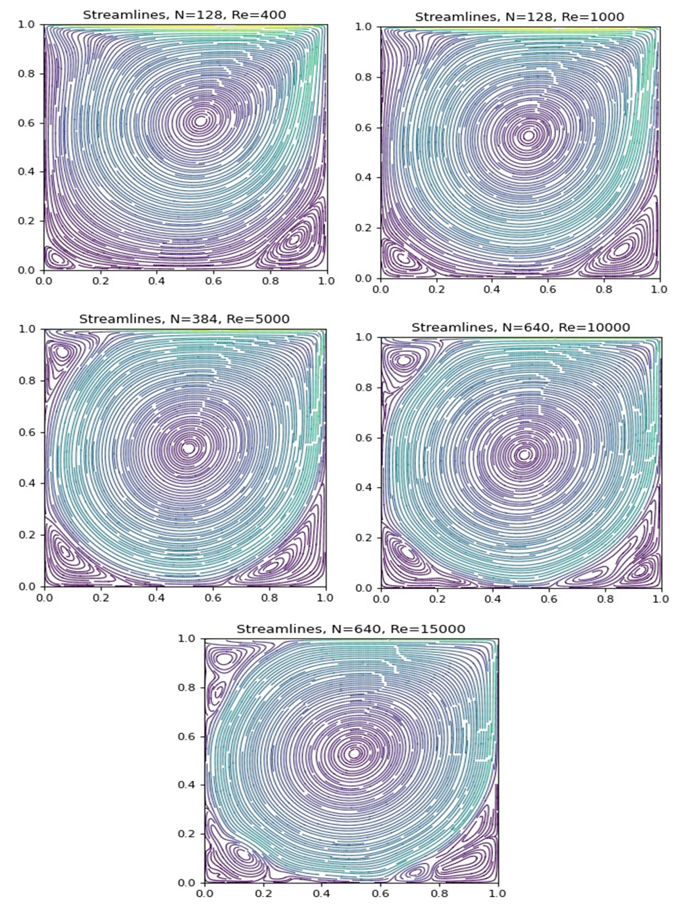
Figure 1. Plots of stream function for various Re. N on title denotes NxN grid requirement

The streamline pattern in the cavity is similar to that previously reported [11] by finite volume method [10] and various other methods [7,9,11,12,4]. Initially two corner vortices appear on the lower wall. The primary vortex gets little sheared in the lid driven direction to right. At Re =5,000, a tertiary vortex appears at the top left corner of cavity. At Re=10,000, another lower corner vortex appears on the right side, the other vortices appear to enlarge, the primary vortex shift more to the center of cavity and top left corner vortex gets bigger. At Re = 15,000, more top left corner and lower wall corner vortices appear, the top corner vortex gets bigger and spreads downwards.

The centerline u and v components of velocity, shown in Fig. 2, correlates pretty well with Ghia et al [4] data. The K in title is same as Ar. The Re 15,000 curve is new and no data is available as per our current knowledge.

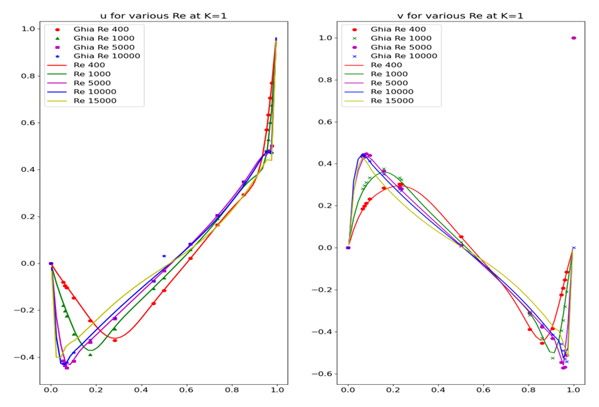
Figure 2. Mid Plane velocity prediction and correlation with bench mark data

A viscosity counteracting approach [14] was used to analyze square cavity flows up to Re = 60,000. Here a small viscosity was added to the dissipation term and was later subtracted as forcing source term. Authors were able to run up to Re =60,000 with very low 200x200 lattice grid density. Presently we use increasing grid density in our code to solve the problem.

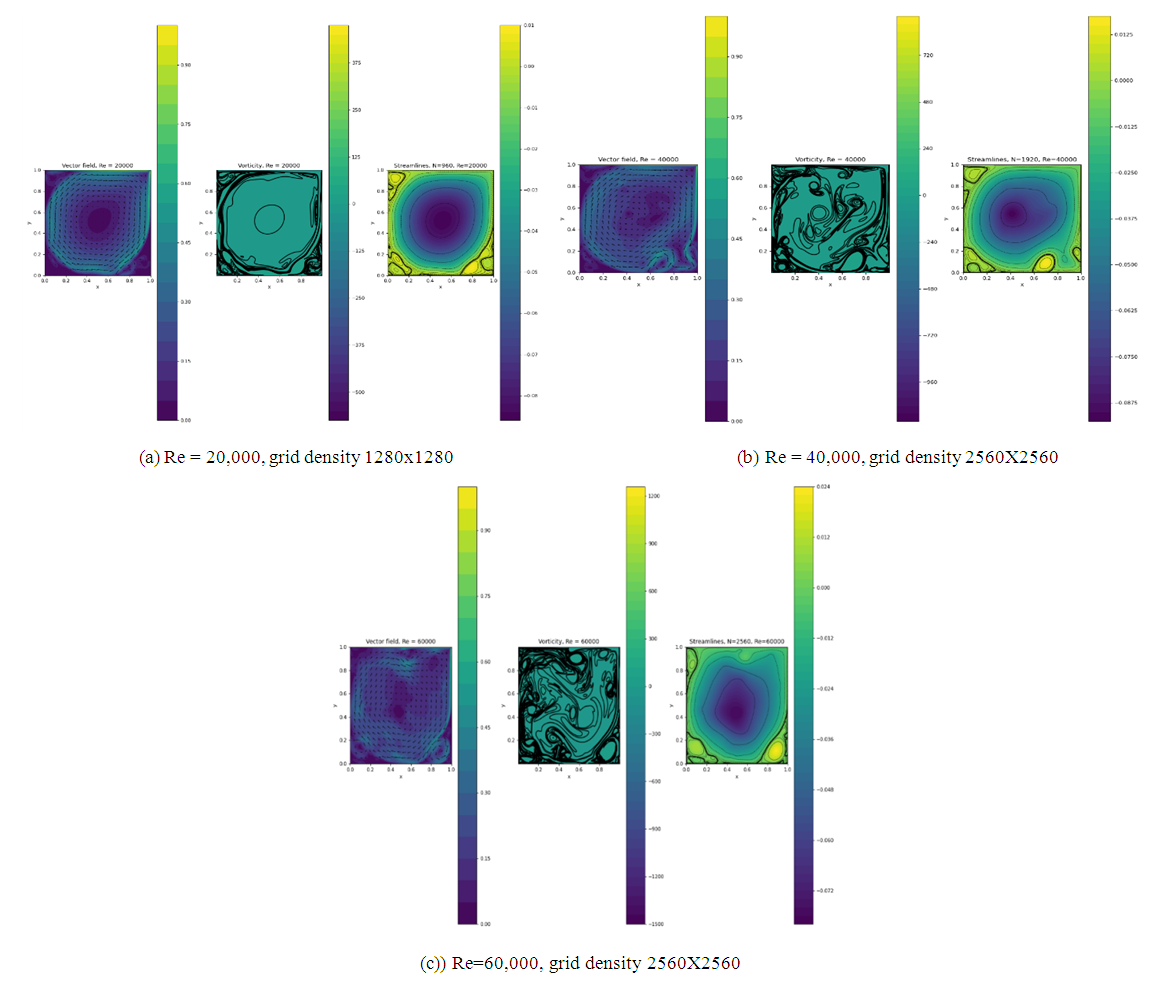
Figure 3. Total velocity, vorticity, and streamlines for several Re

The predicted streamlines are similar to those in ref. [14]

Case 2: Deep Cavity Flow Investigation

The present code [9] can be run for many deep cavities without any modification. The aspect ratio is defined as Ar (or K) = Height/width of the cavity. The grid point distribution will be N times (NxAr). This keeps grid cells evenly distributed. The run times increase with increasing depth (Ar). Since the code is gpu vectorized, most of the high Re >=10,000 were run on Google’s Collaboratory. The platform provided limited access to their Tesla 16 GB gpu. The program runs three to four times faster on gpu compared to cpu only machines. To run in cpu mode, trivial code modifications were required.

Although the investigation can be carried out for any realistic cavity aspect ratio and Re, presently the results were obtained only for aspect ratio Ar=1.5, 4 and 6. Previous investigations [7,15] reported results of Re up to 5,000 and Ar up to 4.

A: Results for aspect ratio Ar = 4

In the following plots, three sets of data are presented for each Re. First is total velocity, second the vorticity and third the streamlines. The magnitude of these data is shown in the scales to their right. Due to space limitations, the titles and scales are not visible, but can be enlarged with usual mouse clicks.

For Re = 400, there is a strong main vortex close to the moving wall. The other three vortices are pretty weak and swirl in the same direction as the top main vortex. Total velocity also shows similar pattern. The vorticity is also constrained in similar way. Up to Re = 5,000, the lower wall vortices grow in size and move upwards. The vortex below the main swirls in opposite direction. The lower two vortices are pretty weak in strength. For Re >= 10,000, the strong main vortex introduces a counter swirling vortex below it, followed by weaker vortices. The number of vortices increased from four to five. The results are consistent with those observed in previous investigations [7,15,5].

Figure 5 shows the mid-section u and v velocity components. Since no comparison data exist publicly, no correlations are attempted. The Re 15,000 profile seems erratic as the laminar flow seems to breakdown as indicated in Fig. 4(e). The swirl direction can be interpreted from this diagram as the centerline velocity passes through eye of the vortices.

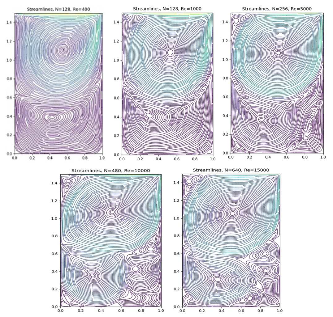
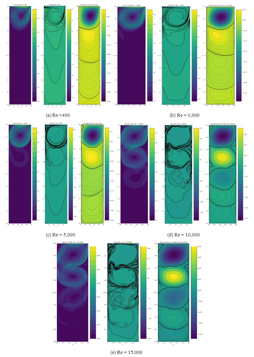
Figure 4. Plots of total velocity, vorticity and stream function for various Reynolds numbers and Ar = 4

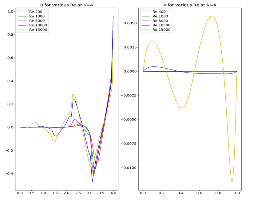
Figure 5. Mid Plane velocity predictions for Ar = 4

B: Results for aspect ratio Ar = 1.5

This aspect ratio cavity has been investigated by several authors [5,7,15] for modest Reynolds numbers up to 5000. Here we will analyze for our base line Re = 400, 1,000, 5000, 10,000, and 15,000 respectively.

Figure 6. Plots of stream function for various Re

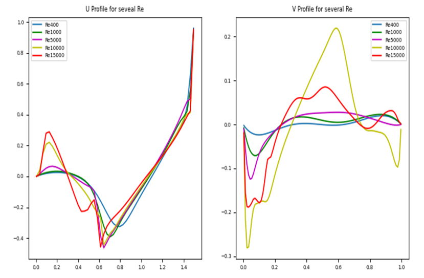
Figure 7. Mid Plane velocity predictions for Ar = 1.5

The bifurcation of the cavity flow regime with two vortices have been well documented [7,5,15]. Further evolution of secondary corner vortices for Re> 1,000 shows that many new vortices in the lower wall corner and top left wall corner region emerge. Once again the flow gets chaotic at Re 15,000. The v- velocity distribution also shows unsteady behaviour at such high Reynolds numbers.

C: Results for aspect ratio Ar = 6

This aspect ratio cavity has not been investigated by any author as per our knowledge. Here we will analyze it for our base line Re = 400, 1,000, 5,000, 10,000, and 15,000 respectively.

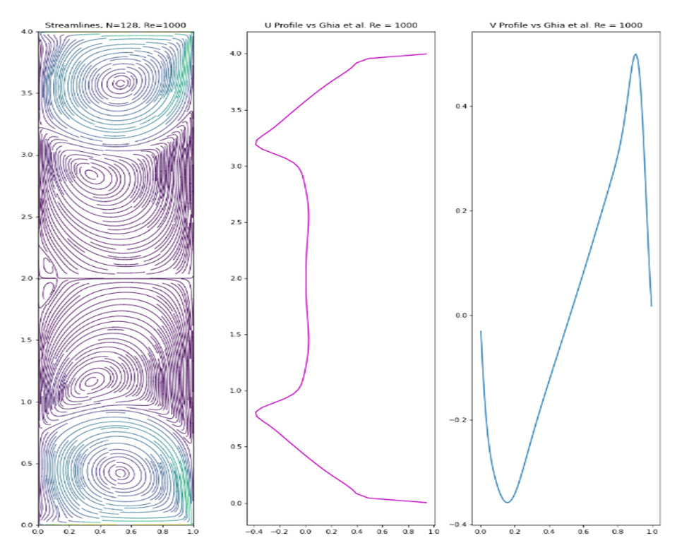
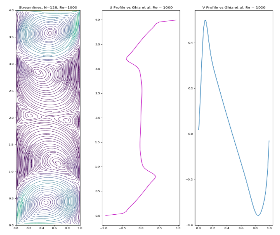
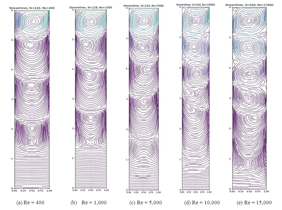
Figure 8. Streamlines predictions for Ar = 6

The streamlines plot up to Re = 1,000 shows a strong top vortex close to the moving wall, followed by three weak vortices, and a nearly stationary region at the bottom wall due to the depth of the cavity. As the Reynolds number increases further, the number of vortices increase and move upwards. The velocity distribution shows more chaotic variation for Re = 15,000.

The mid plane velocity components are shown in Figure 9. The u component shows that most of the vortical activities are confined above 30% of the cavity height. The v component values below Re 1,000, are pretty small compared to Re = 15,000 values.

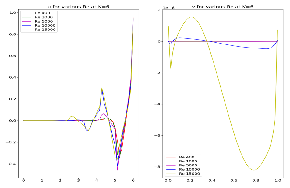
Figure 9. Mid Plane velocities predictions for Ar = 6

D: Overall Effect of Aspect Ratio:

The effect of Aspect ratio on the mid plane velocities for various Ar is shown for Re = 1,000 in Fig. 10. The vertical axis is normalized with characteristic length Ar. With increasing Re, the main vortex moves closer to the top moving wall. The mid u component of velocity rises steeply from minimum close to bottom wall to the lid velocity at the top wall with increasing aspect raio. The v component of velocity shows expected variation.

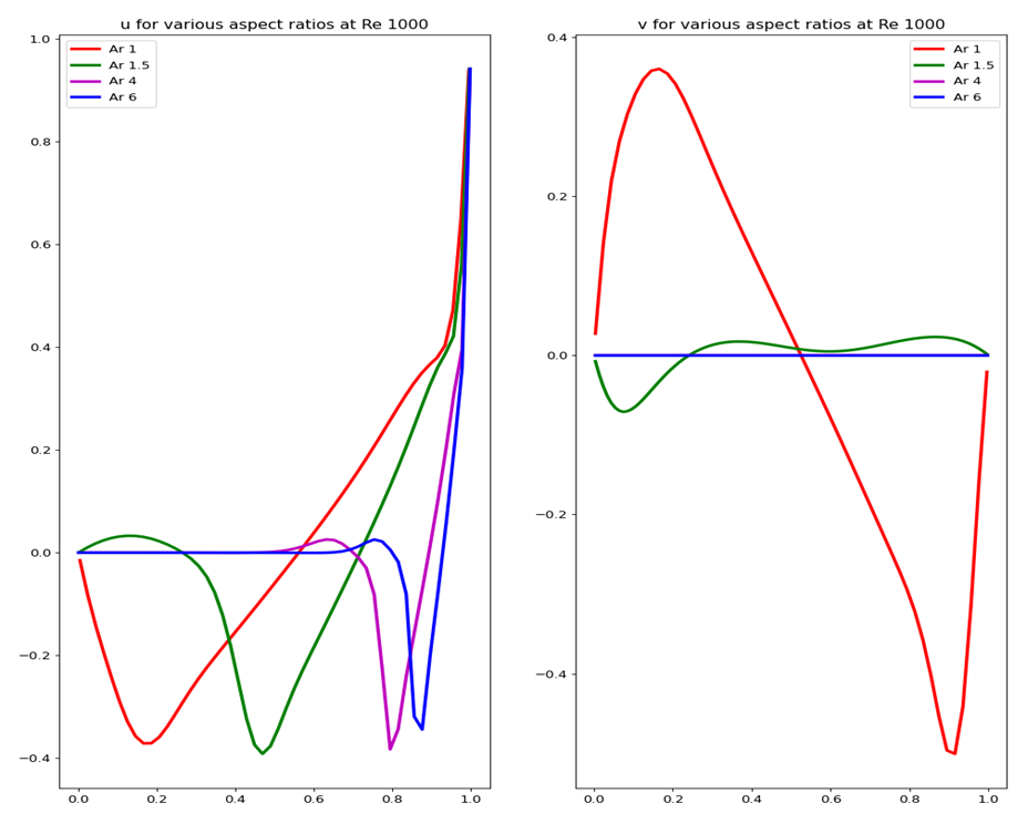
Figure 10. Mid Plane velocity predictions for various Ar and Re = 1000

E: Effect of slip motion of walls.

With a little modification, the cavity flow can be analyzed for any Ar. The bottom wall can move in the same or opposite direction to that of the top wall. We chose Ar = 4 this purpose, The following Figure 11 shows the affect in cavity when walls are moving in the same direction. The vortices clearly get divided by the center plane with symmetrically reflecting vortices near the top and bottom wall. Even the little mid plane small shear eddies are symmetrically located. Similar effect was shown for cavity with Ar=1 in our previous work [11].

Figure 11. Walls moving in same direction

The following Figure 12 shows the cavity flow when the walls are moving in the opposite direction. The mid plane develops a large shearing vortex. The vortices near top and bottom walls are nearly symmetric reflection. Similar effect was shown for cavity with Ar=1 in our previous work [11].

Figure 12. Walls moving in opposite direction

The mid plane velocity variations follow the expected pattern.

3. Conclusions

The present LBE solver with TRT scheme seems to be capable of running the cavity flow problem from moderate to high Reynolds numbers. For square cavity, results shown for Re up to 60,000 exceed those of previous investigations up to 5,000. The results compare well with existing benchmark data for square cavity flow. The code was very stable and can run low to high aspect ratio cavity flows. The velocity data will be put in https://github.com/narain42/Poission-s-Equation-Solver-Using-ML as velocity data folder for future correlation purposes by inspiring new authors.

References

[1]  Batchelor, G.K., “On Steady Laminar Flow with Closed Streamlines at Large Reynolds Numbers”, J. Fluid Mech., 1956, 1: 177-190.
[2]  AbdelMigid T.A., Saqr K.M., Kotb M.A., Aboelfarag A.A., “Revisiting the lid-driven cavity flow problem: Review and new steady state benchmarking results using GPU accelerated code”, Alexandria Engineering Journal, Oct 15, 2016.
[3]  Burggraf, O.R., “Analytical and numerical studies of the structure of steady separated flows”, J. Fluid Mech., 1966, 113-151.
[4]  Ghia U, Ghia KN, Shin CT., "High- Re solutions for incompressible flow using Navier–Stokes equations and a multigrid method.", J Comput Phys 48: 387, 1982 [5].
[5]  Lin L.S., Chen Y.C., Lin C.A., “ Multi relaxation time lattice Boltzmann simulation of deep lid driven cavity flows at different aspect ratios”, Comput. Fluids., 45(2011), 233-240.
[6]  Wikipedia, “Lattice Boltzmann Method”, , 2022.
[7]  Patil, D.V., Lakshimsha, K.N., Rogg, B., “Lattice Boltzmann solutions of Lid driven flow in deep cavities”, Computers and Fluids, 35, (2006), 1116-1125.
[8]  Bhatnagar, P. L.; Gross, E. P.; Krook, M. (1954-05-01). "A Model for Collision Processes in Gases. I. Small Amplitude Processes in Charged and Neutral One-Component Systems". Physical Review. 94 (3): 511–525.
[9]  Burrows Travis, "2D Lid Driven Cavity with GPU in Python with pyOpenCL, Lattice Boltzmann Method”, pyOpenCL-LBM, GitHub, June 11, 2020.
[10]  Boria Servan -Cmas Frank, T-C Tsai, “Two-relaxation-time lattice Boltzmann method for the anisotropic dispersive Henry problem”, , Feb 2010.
[11]  Henrik Spietz, "2D Navier-Stokes Solver for the square cavity flow using the finite-volume method", spietz / DNSSolver in GitHub, May 4, 2019.
[12]  Narain, J.P., “Lid Driven Cavity Flow: Review and Future Trends”., Am. J. of Fluid Dynamics, vol, 12, No. 1, 2022, pp 1-15.
[13]  Brownlee, R.A., Levesley, J., Packwood, D., and Gorban, A.N., “Add-ons for Lattice Boltzmann Methods: Regularization, Filtering and Limiters”, Progress in Comp. Physics, Vol. 3, 2013, 31-52.
[14]  Cheng, Y. and Zhang, H, “A viscosity counteracting approach in the lattice Boltzmann BGK model for low viscosity flow: Preliminary verification”, Computers and Math with Applications, vol 61, (2011) 3690-3702.
[15]  Kumar A, Agrawal, S.P., “ Mathematical and simulation of lid driven cavity flow of different aspect ratios using single relaxation time lattice Boltzmann technique”, Am. J. of The. And App. Stat., vol 2(3), 2013, pp 87-93.