1. Introduction

The lid driven flow inside a square cavity has drawn considerable numerical and experimental interest for decades. Theoretically, Batchelor [1] pointed out that lid driven cavity flows exhibit almost all the phenomenon that can possibly occur in incompressible flows: eddies, secondary flows, complex flow patterns, chaotic particle motions, instability, and turbulence. Practical applications are in material processing, dynamics of lakes, metal casting, galvanizing and some airport runways. Tamer et. al. [2] have given a concise review of the developments of various numerical schemes, starting from finite-difference [3,4], finite-volume [5] to Lattice Boltzmann(LB) methods [6,12,13,14]. Although so many remarkable methods have been outlined in the review [2], we will use a modified version of finite-volume code [7] to present several scenarios and compare them with current LB method. The physics informed deep learning (PINN)method [8] revolutionized neural network application to several fluid-dynamics problems. We will use two newer PINN methods [9,10] to analyze and assess the current status of the PINN scheme. The deep cavity flow with aspect ratio greater than one has also drawn considerable attention using LB scheme [12] as well as Fluent commercial software [16]. We will show deep cavity results with the finite volume and PINN solvers. The present PINN methods can not analyze high Reynolds number scenarios. Some insight into this problem will be presented.

2. Discussions

We will start with a finite volume solver. During our assessment, it was found to be superior to basic finite difference methods and gave consistently remarkable results compared to results from any published work. It is quite fast, takes only a few seconds for low Reynolds numbers and increasing minutes for high Reynolds number flows on a basic home computer. The stream function or psi, vorticity and pressure equations for a two-dimensional incompressible flow are given by [11];

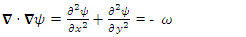(1)

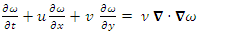(2)

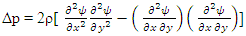(3)

Where is the stream function, is the vorticity, p is the pressure, and ρ is the density.

The cavity problem will be solved for two vertical stationary walls, and with top wall moving with a velocity u0=1. The slip conditions for the bottom wall will be stationary, or moving in same direction with velocity u0=1, or in opposite direction with velocity uo=-1. A schematic cavity is shown as follows;

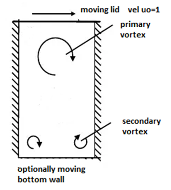Sketch 1. A cavity with top and moving wall concepts

The boundary conditions are:

(4)

(5)

On the top wall:

(6)

Where n is a direction normal to the wall. For a moving wall, the boundary condition (6) is obtained by Thomas expansion of eq(5). Similar equation can be obtained for moving bottom wall. The pressure calculation and boundary conditions are described in ref [11]. The symbols(i,N) denote the grid points of the cavity (N,N).

Case A: The flow inside a square cavity with top wall moving with velocity u0 to the right:

The grid point distribution study showed that a grid of 41x41 points is adequate for the analysis. Since a few papers have indicated, a grid of 81x81 should be optimum for any analysis, we have selected this grid of equidistance points in a unit size cavity. The Reynolds number is defined as Re = u0 L / 𝜈, where L is 1 for unit cavity. Here 𝜈 = 1/Re since u0=1. Most of the publications report the results for moderate Reynolds number of 100 and 400, and for high Reynolds numbers of 1000, 3200, and 5000. We ran all the Reynolds numbers and have shown important flow variables, psi, vorticity, pressure, u and v velocity components.

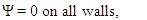
Figure 1. Plots of stream function for various Reynolds numbers

The following figure shows the vortex pattern inside the cavity from a LB solver [12]:

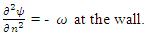
Figure 2. Plots of stream function for various Reynolds numbers from a Lattice Boltzmann solver [12]

The accuracy of the present finite volume solver is as good as that of LB solver using particle motion theory. For Re = 100 the streamlines are slightly off from being symmetrical about the middle of the cavity, the streamlines are slightly crowded near the moving lid, where the largest velocities arise, and two separated eddies in the bottom corners are signaled by the two separating streamlines.

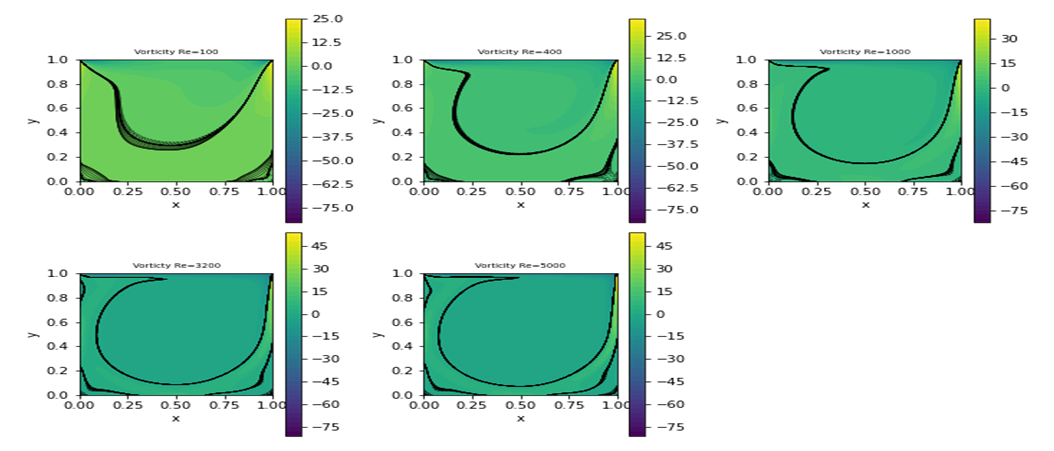Figure 3. Plots of vorticity for various Reynolds numbers from the present fv solver

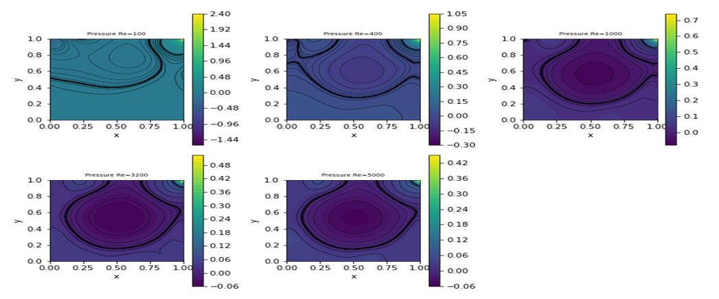Figure 4. Plots of pressure for various Reynolds numbers from the present fv solver

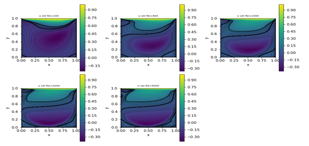Figure 5. Plots of streamwise velocity u for various Reynolds numbers from the present fv solver

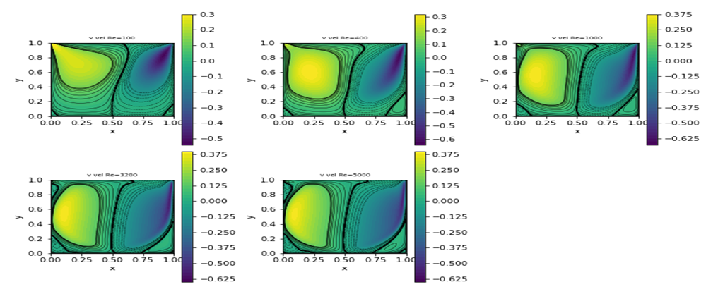Figure 6. Plots of transverse velocity v for various Reynolds numbers from the present fv solver

When the Reynolds number is large (Re >=1000), inertia terms in eq. (2) destroy the reflectional symmetry with respect to middle width of the cavity. The separated vortices at the bottom become stronger. A third separated region is created, for Re greater than 3200, close to the upstream corner of the moving lid near (x, y) = (0, 1). For even higher Reynolds number (Re=5000), the core of the vortex approaches a solid-body rotation with circular streamlines and constant vorticity [1] which can be seen in figures 1, 2 and 4. The velocity profiles become linear in the bulk for high Reynolds numbers of Re=5000 as evidenced in Fig, 7.

Next, we will show rest of the flow variables as they are seldom shown in detail.

The velocity distribution in x-direction is shown in Figure 5. The smallest value (-0.33) and its location agree very well with the results in ref. [17] for Re=400. Near the lid there is a large velocity gradient, the lower left and lower right corner are dead zones. The pressure plot, Figure 4, reveals a low-pressure zone in the center of the major vortex and in the left upper corner. The right upper corner is a stagnation point for the x-component of the velocity and is characterized by a significant pressure build-up.

A comparison of mid-section u and v velocities for all Reynolds number with reported test and analytical data [2] are shown below:

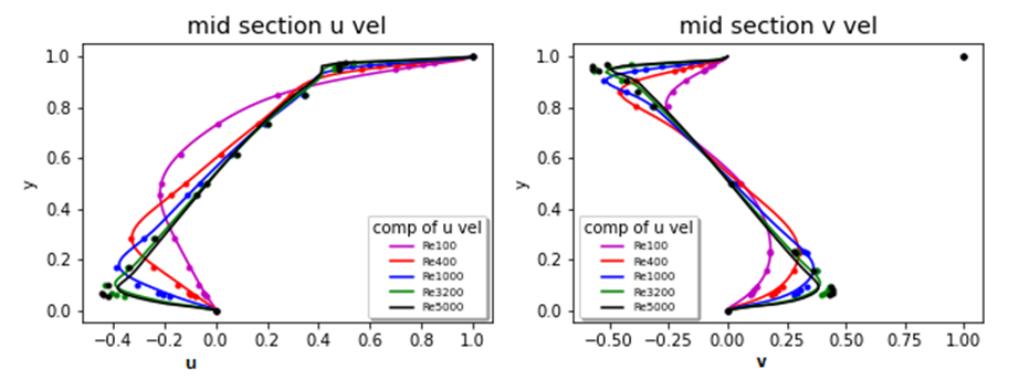Figure 7. A comparison of centerline u, v velocities for all analyzed Reynolds numbers

The extensive display of results may seem redundant, but has not been published in one paper before. It will serve as future reference in computational fluid dynamics (CFD) studies.

Case 2: Top and Bottom walls moving in opposite direction:

The solution of cavity flow with top and bottom walls moving is in general not unique. The non-uniqueness of the two-dimensional double-lid-driven cavity flow was studied more systematically by Albensoeder et al. [18]. They found up to seven different two-dimensional steady flow states for the same boundary conditions. Multiplicity is observed for condition when both walls move either in parallel or anti-parallel direction. Finite volume solver reproduces a case of strongly merged vortex flow.

Figure 8 shows the solution from a LB solver and Figure 9 shows the corresponding solution from the present finite volume solver. The solution matches exactly even in finer details.

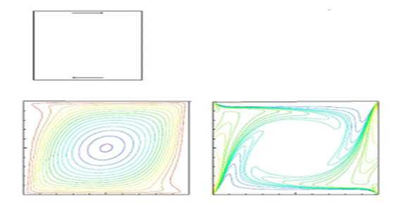Figure 8. Plots of cavity configuration, stream function and vorticity at Re=400 from a Lattice Boltzmann solution paper [13]

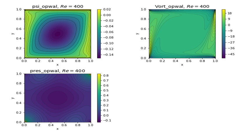Figure 9. Plots of stream function, vorticity, and pressure at Re=400 from a present finite volume solver

Result for Re=5000 is shown in Figure 10. No plots are available from ref. [13]. A look at the velocity plots will also be interesting. Figure 11 shows such a plot.

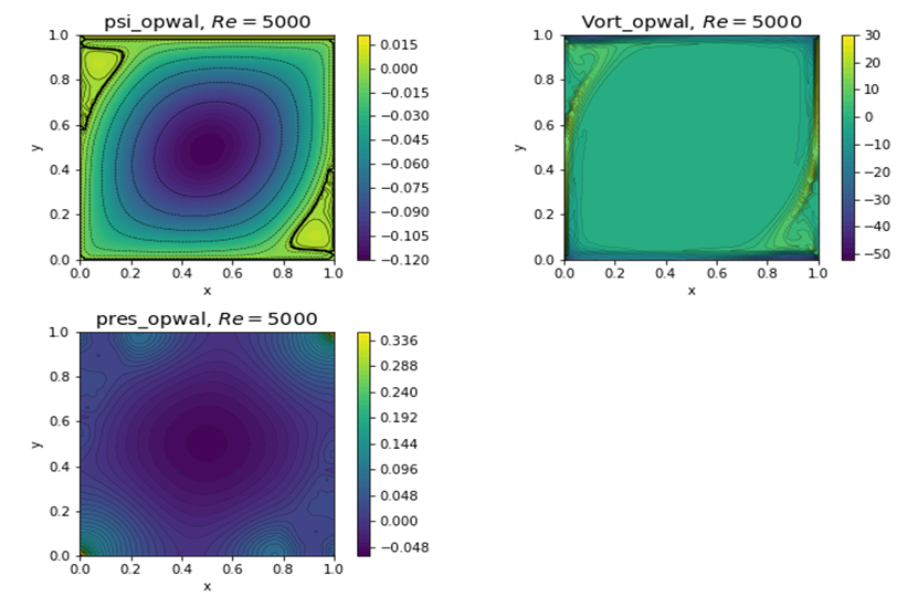Figure 10. Plots of stream function, vorticity, and pressure at Re=5000 from a present finite volume solver

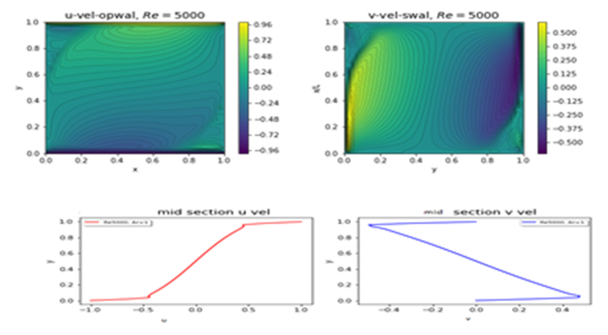Figure 11. Plots of u and v velocity components and their mid-section values at Re=5000

Case 3: Top and Bottom walls moving in the same direction:

There has been considerable research interest for this slip configuration. Since walls are moving in the same direction with the same velocity, the resulting strong vortex has stabilizing effect on the numerical stability. This results in the faster convergence of solutions. Although results can be obtained for wide range of Reynolds number, we will show a couple at Re=400 and Re= 1000. The fv stands for current finite volume solver in the figure captions.

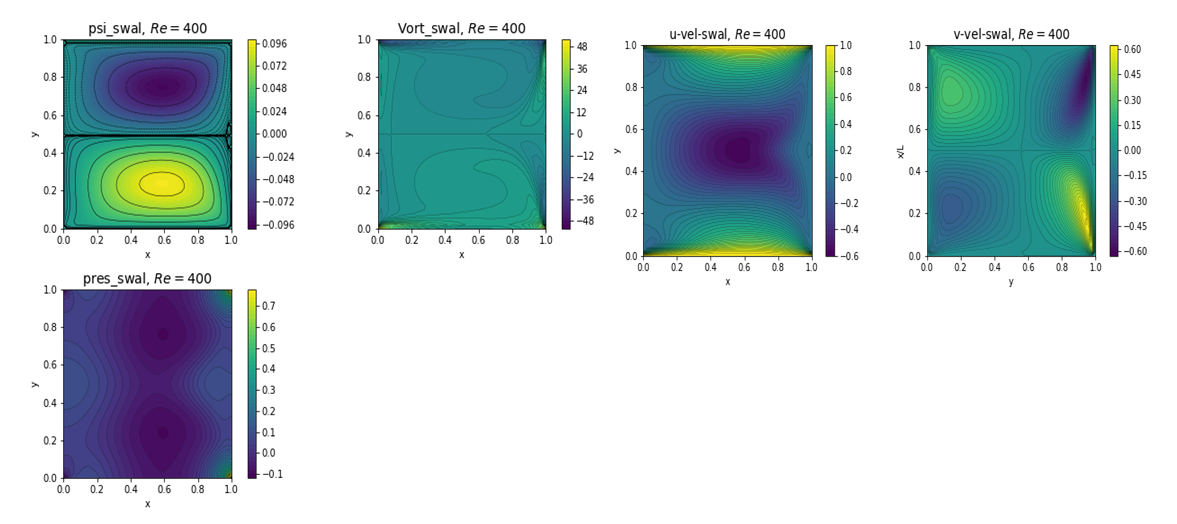Figure 12. Plots of psi, vorticity, pressure, u and v velocity for Re=400 from fv solver

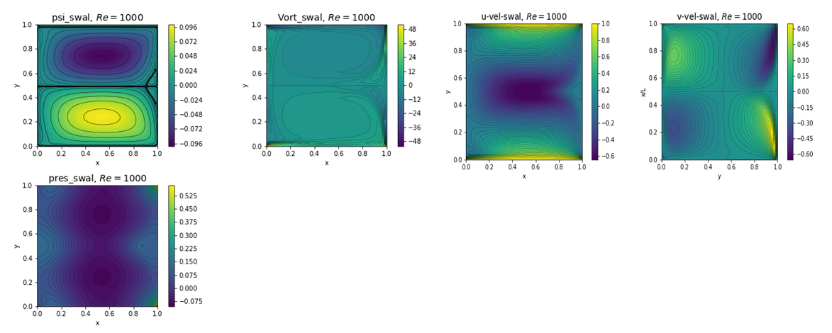Figure 13. Plots of psi, vorticity, pressure, u and v velocity for Re=1000 from fv solver

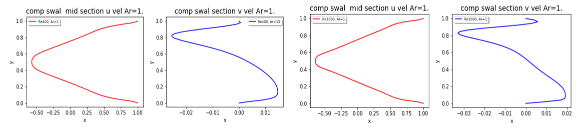Figure 14. Plots of u and v velocity components at mid-section for Re=400 and Re=1000 from fv solver

Case 4: Deep Cavity Flow Investigation using finite volume solver (fv):

For shallow cavities with aspect ratio aspect ratio Ar = Height/Width <<1 and small Reynolds numbers the streamlines become nearly parallel, except for the turning zones near the walls. For deep cavities (Ar>=1), on the other hand, the flow separates repeatedly. The main vortex, whose core develops circular streamlines for high Reynolds numbers, drives another weaker separated and counter-rotating vortex, and so on.

The present fv solver is numerically for a square cavity, i.e. a nxn grid where n is the size index for the grid (like 81 points used here). However, it does not necessarily mean that cavity size be a unit square. Thus, a cavity of any aspect ratio can be modelled with different grid spacing dx and dy in x and y direction. However, the fv numerical method assumes uniform grid in both x and y direction. Hence a larger aspect ratio like Ar=4 will not work because of large disparity in grid sizes. We will present a case for Re=700 and Ar=2.0 and compare the results with ref. [13]. The walls are moving in the same direction.

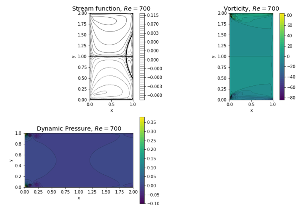Figure 15. Plots of psi, vorticity, pressure, u and v velocity for Re=700, Ar=2 from fv solver

The corresponding results from the LB solver of ref [13] is shown below:

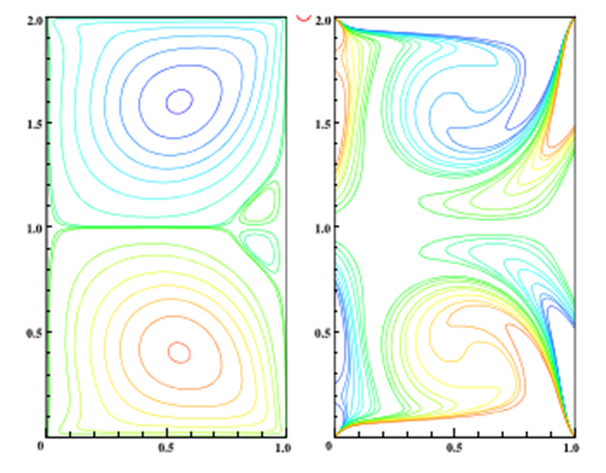Figure 16. Plots of psi, and vorticity for Re=700, Ar=2 from LB method

The slip motion scenario is well modelled by the present fv solver. The bifurcation of stream function at the mid height helps in better prediction. For non-slip case of top wall moving only, the analysis showed slanted bifurcation, which is not supported by other solver [13]. We are working to resolve this issue.

Case 5: Physics Informed Neural Network:

With the advent of Raissi et al [8] work on physics informed neural network (PINN), most of the research relied on his basic principle. One has to have a computational fluid dynamics (CFD) solution to the problem before doing any neural network analysis. Some went out of the box and showed that one does not need either a grid, or a solution to do such an analysis [9].

“The PINN is a deep learning approach to solve partial differential equations. Well-known finite difference, volume and element methods are formulated on discrete meshes to approximate derivatives. Meanwhile, the automatic differentiation using neural networks provides differential operations directly. The PINN is the automatic differentiation-based solver and has an advantage of being meshless.

In addition, an effective convergent optimizer is required to solve the differential equations accurately using PINNs. The stochastic gradient descent is generally used in deep learnings, but it only depends on the primary gradient (Jacobian). In contrast, the quasi-Newton based approach such as the limited-memory Broyden-Fletcher-Goldfarb-Shanno [14] method for bound constraints (L-BFGS-B) incorporates the quadratic gradient (Hessian), and gives a more accurate convergence.”

The application of this concept for a flow inside a cavity with upper wall moving with unit velocity provided the following solution. The equations are similar to finite volume stream function, vorticity, and pressure formulation. The results for Re 100 and 400 are shown below.

The results show excellent comparison with fv solutions presented earlier in Figures 1 thru 6 for Re=400. However, there is a major problem for simple home pc users. The (L-BFGS-B) solution with 200000 iterations take more than 11 hours on a 16 GB Intel 7-6700 cpu machine. The alternative to this is to use Adam optimization [15], for 90% of 5000 iterations, followed by 10% with (L-BFGS-B) optimization. The above results were run and duplicated within 3 hours on a basic computer.

The higher Reynolds number cases of Re = 1000, 3200 and 5000 could not be run. According to author, the following is the explanation.

“We verified that PINN algorithm cannot get an ideal convergence for complex phenomena such as high Reynolds flow and high-dimensional equation. Deep neural networks potentially represent their solutions, but localized ones constrict even though we use quasi-Netwon method.

This problem is a challenge to overcome for implementing PINN application.”

Figure 17. Plots of psi, p, u, v, and u-, v- velocity components at mid-section for Re=100

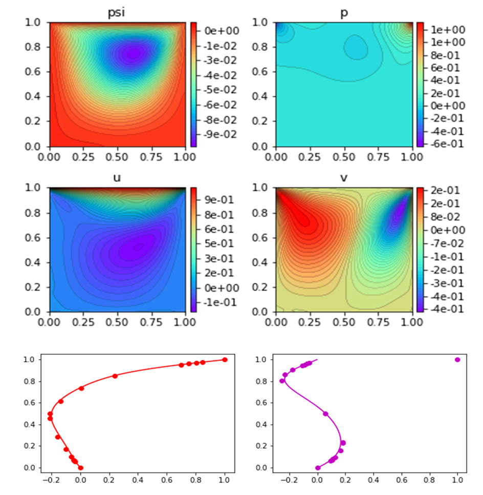
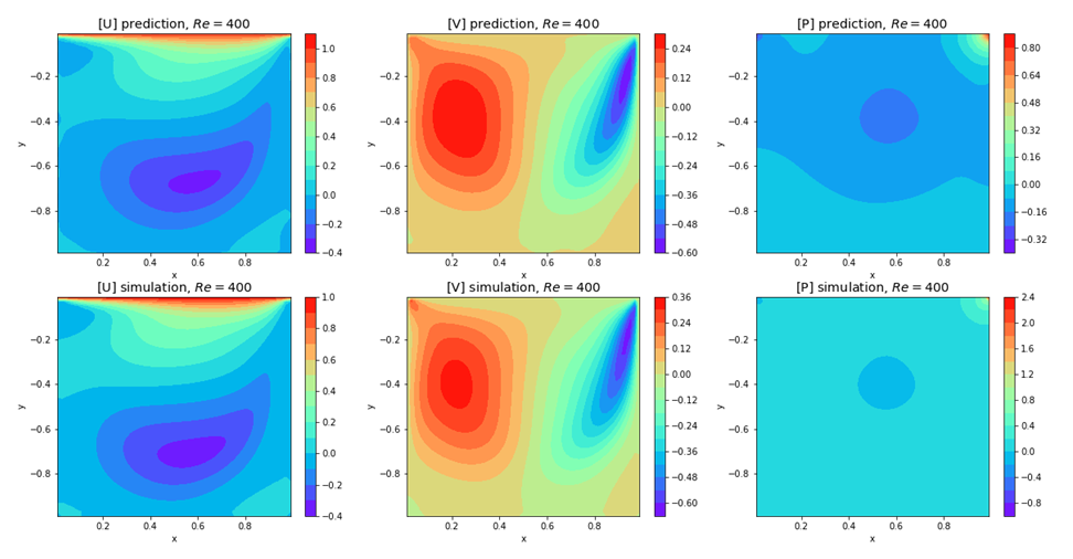
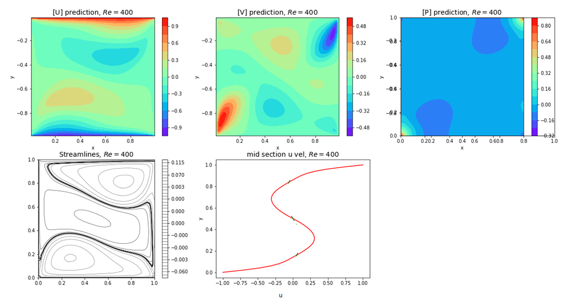
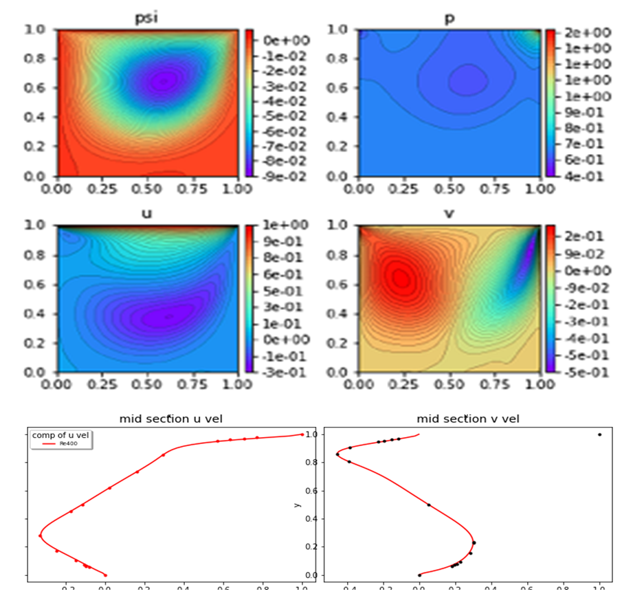Figure 18. Plots of psi, p, u, v, and u-, v- velocity components at mid-section for Re=400

Case 6: CAN-PINN: A fast physics-informed neural network based coupled-automatic-numerical differentiation method [10]:

“In this study, novel physics-informed neural network (PINN) methods for coupling neighboring support points and automatic differentiation (AD) through Taylor series expansion are proposed to allow efficient training with improved accuracy. PINNs constrain their training loss function with ordinary and partial differential equations, to ensure outputs obey the governing physics. The computation of differential operators required for loss evaluation at collocation points are conventionally obtained via automatic differentiation. Although AD method has the advantage of being able to compute the exact gradients at any point, such PINNs can only achieve high accuracies with large numbers of collocation points—otherwise they are prone to optimizing towards unphysical solution. To make PINN training fast, the dual ideas of using numerical differentiation (ND)-inspired method and coupling it with AD are employed to define the loss function. The ND-based formulation for training loss can strongly link neighboring collocation points to enable efficient training in sparse sample regimes, but its accuracy is restricted by the interpolation scheme. The proposed coupled-automatic-numerical differentiation framework—labeled as can- PINN—unifies the advantages of AD and ND, providing more robust and efficient training than AD-based PINNs, while further improving accuracy by up to 1-2 orders of magnitude relative to ND-based PINNs. For a proof-of- concept demonstration of this can-scheme to fluid dynamic problems, two numerical-inspired instantiations of can- PINN schemes for the convection and pressure gradient terms were derived to solve the incompressible Navier-Stokes (N-S) equations. Theoretical analysis shows that the proposed can-schemes have smaller dispersion and dissipation errors than the baseline ND-based schemes. The superior performance of can-PINNs is demonstrated on several challenging problems, including the flow mixing phenomena, lid driven flow in a cavity, and channel flow over a backward facing step. The results reveal that for challenging problems like these, can-PINNs can consistently achieve very good accuracy whereas conventional AD-based PINNs fail.”

The code was provided on GitHub. Here again, the converged results were obtained only for moderate Reynolds numbers. We will show only results for Re=400 to preserve some space.

Figure 19. Plots of u, v, and p for Re=400

This is true PINN method where a known simulation CFD solution (simulation) is provided for predictive training sample. Presently it was discovered that one does not need a CFD solution for the analysis. One can use its own grid to start the solution. The predictive solution can be totally random arrays, zero arrays, unity arrays, or even any flow variable solution fitting the grid. The following shows the solution with random simulation arrays.

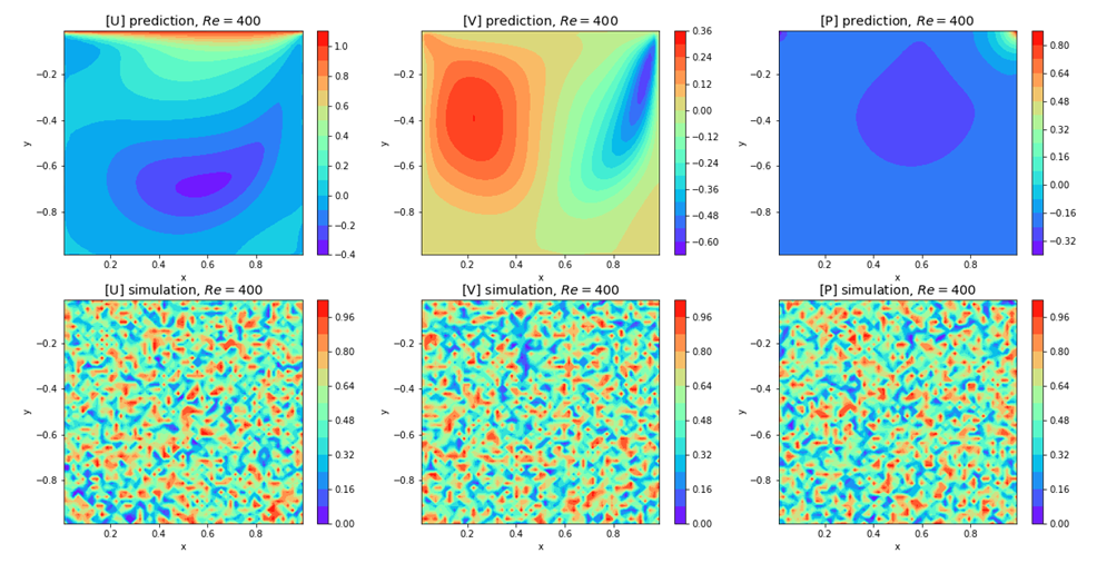Figure 20. Plots of u, v, and p for Re=400 with random predictive samples

The streamline and the comparison of velocities with known results are shown below;

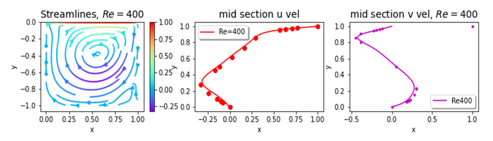Figure 21. Plots of psi, u, v at mid sections for Re=400

All these results were obtained with Adam optimization and 5000 iterations. Run time was within 3 hours on basic home pc. The results compare well with results shown in Figures 1 thru 6 and 18 by different methods. This well documented code provides clear places where boundary conditions can be changed. We were able to run with top and bottom walls moving in same and opposite directions.

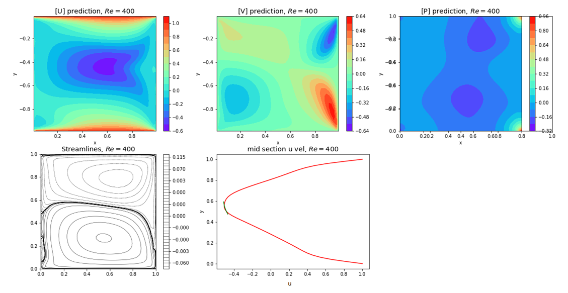Figure 22. Plots of u, v, p, psi and u-, v- velocity components at mid-section for Re=400 and for top and bottom walls moving in same direction with unit velocity

Figure 23. Plots of u, v, p, psi and u-, v- velocity components at mid-section for Re=400 and for top and bottom walls moving in opposite directions with unit velocity

Attempts to run at high Reynolds number greater than or equal to 1000 were futile.

Case 7: Deep cavity investigation:

The flow inside deep cavity of aspect ratio (Ar) = height/width has been investigated for the values of 1.5 and 4 in various references [12,13,14,16]. Here we will show results for Reynolds number, Re=400. The results are shown for upper wall moving to the right with unit speed, whereas the lower wall may be stationary, or moving in the same, or opposite direction relative to the upper wall.

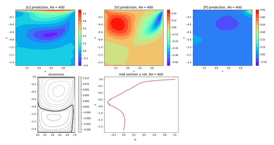Figure 24. Plots of u, v, p, psi and u-, v- velocity components at mid-section for Re=400 and for Ar=1.5

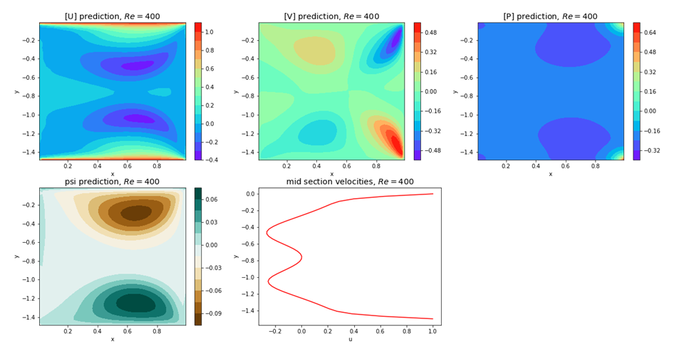Figure 25. Plots of u, v, p, psi and u-, v- velocity components at mid-section for Re=400 and for Ar=1.5, and top and bottom walls moving in same direction

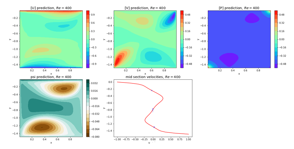Figure 26. Plots of u, v, p, psi and u-, v- velocity components at mid-section for Re=400 and for Ar=1.5, and top and bottom walls moving in opposite direction

The results are consistent with those in previous published work [12,13,14]. The results for Ar=4 did not show favorable results for the same reasoning as that in fv solver.

Case 8: High Reynolds number problem:

Looking at all these figures, it becomes clear that at high Reynolds number, the viscosity decreases sharply, and the convergence becomes difficult. The high frequency errors dominate near separation points in such cases. If in some way we can introduce more dissipation or artificial viscosity without affecting the governing equations and the boundary conditions, we may be able to get a solution.

One such case was the cavity top and bottom walls moving in the same direction at Re=1000. The results are shown below.

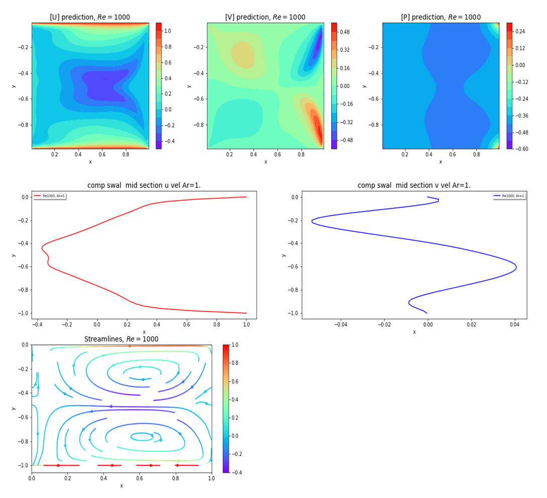Figure 27. Plots of u, v, p, psi and u-, v- velocity components at mid-section for Re=1000 and for top and bottom walls moving in the same direction with unit velocity

Figure 28. Plots of u, v, p, psi and u-, v- velocity components at mid-section for Re=1000 and for top wall moving with half speed

The results in Figure 27 compare well with the fv solutions for Re=1000 shown in Figures 13 and 14. It becomes more intuitive at this point that if one can induce more vortical dissipation, one can overcome this high Re barrier. However, the present hypothesis did not go beyond Re=1000.

For a cavity with only top wall moving, above concept can be applied if the wall speed is reduced. For the top wall moving at speed of u0=0.5, a solution can be achieved at Re=1000. The results are shown in Figure 28.

The codes for all the present work are available at narain42/Poisson-s-Equation-Solver-Using-ML on GitHub.com. Only the modified CAN-PINN will be delivered. The finite volume code [7] and the pinn-cavity codes [9] are available in referenced GitHub repository.

3. Conclusions

The present finite volume solver seems to be capable of running the cavity flow problem from moderate to high Reynolds numbers. The results compare well with finite volume and LB results which seem to be a good benchmark for cavity flow analysis. A few physics informed neural network works were reviewed. The use of external CFD solution seems to be unwarranted. Since machine learning is based on random simulations, so random simulation is the best way to go. The ability of PINN codes to run at high Reynolds number was examined. A few cases were run for Re=1000 where additional viscosity was induced by wall motions. This was just a preliminary concept. More work needs to be done by Academicians to overcome this issue.