1. Introduction

A confluence is a place where two flows with the same or different characteristics merge. The flow may be natural or artificial. Specifically, two or more water bodies (rivers, streams, lakes, or canals) may collide, conflux, or merge to form a new single flowing water body. When two rivers merge to become the source of a new one, in some cases, the waters may mix, as in the confluences of Rivers Ilz, Danube, and Inn in Passau, Germany; Jialing and Yangtze in Chongqing, China; Thompson and Frazer in Lytton, British Columbia, Canada; Benue and Niger in Nigeria. In other cases, they may not mix, as in the confluences of Rivers Ohio and Mississipi at Cairo, Illinois in the USA; Rio Negro and Rio Solimoes, near Manaus, Brazil; see [1].

The merging of rivers takes many forms. In some, a small river (the lateral flow) enters a large one (the main flow) to form an open channel flow, as in tributaries; in others, two non-parallel rivers flowing in approximately the same direction meet at a point to form a single stream. The merging rivers rising from mountains whose gradients, the chemical composition of the source rocks, and environmental climatic conditions are different are bound to have different velocities, chemical compositions, temperature and colours, geological properties, etc. Similarly, river confluence flows are characterized by significant changes in flow dynamics, sediment transport, and bed morphology.

Merging flow problems have been studied in a diversified manner. Some studied the merging flow of blood in arteries, and many others, the confluence flow of rivers and streams. On merging blood flow, [2] considered the flow through a straight channel with an upstream splitter plate; [3], neglecting the effects of pulsatility, investigated a two-dimensional merging blood flow in a basilar artery using geometrical transformation, conformal mapping, and numerical approaches. More so, on a general note, [4] numerically examined a steady two-dimensional asymmetric merging flow of micro-polar fluid in a rectangular channel. Similarly, the merging flow of two rivers has been studied from different perspectives. Some studied it ecologically [5], some hydro-dynamically [6] - [14]); some sedimentologically ([15] - [17]); some through laboratory experiments ([18], [19]), and others by field survey ([20] - [23]). Importantly, on a hydro-dynamic review of reports, [24] studied the flow dynamics of an open confluence flow for several merging angles and discharge ratios, and noticed that the flow has six hydro-dynamic regions: flow deflection, flow stagnation, flow separation, maximum velocity, shear layer, and flow recovery; the flow is characterized by helical flow cells. [9] studied the mixing processes in laboratory and field confluences using a 3-D Re-Normalization Group Theory (RNG) turbulence model and showed the difference between concordant (equal bed levels) and discordant (uneven bed levels) rivers, and the effects of the channels curvatures on the flow mixing. [12] investigated the combined hydrodynamic, sediment transport, and mixing processes in large confluences using a field study approach, water quality, and seismic profile measurement, and observed the key hydrodynamic features of large confluences. [14] gave a review of the flow dynamics and sediment transport at open channel confluences, but with a focus on the link between flow dynamics, sediment transport, and bed morphology.

Upon the above reports, it is evident that many of the studies on the confluence flow of rivers were carried out using field surveys, experiments, simulations, and otherwise. This paper presents an analytic model of the hydrodynamic behaviour of the mix-merging flow of two rivers with different flow characteristics. We investigate among others, the effects of some important hydro-dynamic parameters on the flow and transport of bed-loads/sediments.

This paper is organized as follows: section 2 is the Methodology; section 3 is the Conclusion.

2. Methodology

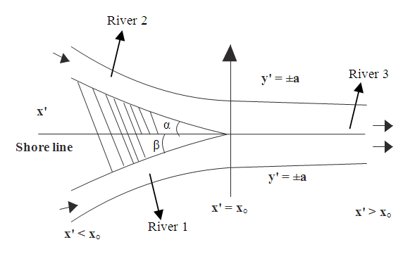Figure 1. A physical model of symmetrical confluxing flowing rivers (α=β)

Figure 1 is a realistic representation of a merging flow of two rivers whose merging angles range from 0<α<90°. In particular, a merging angle of α=90° tends to portray a case where two rivers flowing from opposite directions meet, then clash into a merger.

We consider the confluxing-mixing flow of two rivers whose dependent flow characteristics differ. The modeled problem is formulated based on some physically realistic premises. For example, we assume the merging river channels are symmetrical, the river waters are incompressible, Newtonian, and magnetically susceptible (due to the presence of dissolved/decayed materials, alkaline/salts from the source rocks); the waters are at different levels of concentration, and as such a chemical reaction, which is of a homogenous first-order type (i.e. the reaction is proportional to the concentration) is triggered up; the waters are at different velocities, temperature and concentration such that at mixing they have common flow characteristics; the source rocks and flow channels are porous and non-homogenous such that their permeabilities are anisotropic; the environmental temperature effect is present such that a thermal differential exists between it and the rivers water equilibrium temperatures. Specifically, the environmental/external temperature depends on the radiation from the sun and is usually higher than the ambient temperature of the rivers. Upon this, heat flows into the rivers from their surfaces. Naturally, the absorbed heat interacts with and energizes the water particles, thus accounting for the prescription of the net exchange term in the energy equation. Similarly, combining with other factors, the heat transferred generates convection currents, which is prescribed in the momentum equations.

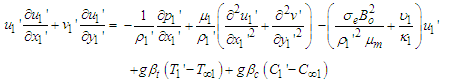
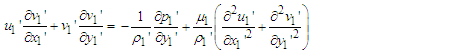
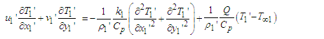
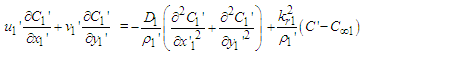
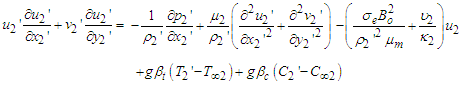
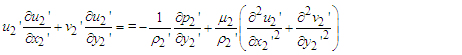
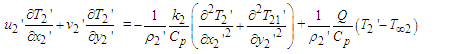
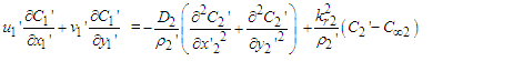
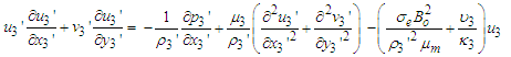
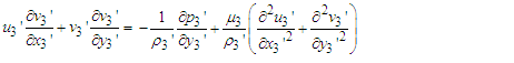
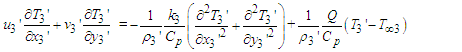
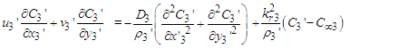
Rivers are planar at the surface. Considering a 2-D case, we assume the velocity is symmetrical about the -axis. Therefore, if and are mutually orthogonal axes and the associated velocity components; and are the concentration and temperature of the waters in the merging channels, and are the equilibrium concentration and temperature of the waters in the merging channels, then by the Boussinesq approximations, the equation of mass balance, momentum, energy, and diffusion guiding the flow are as follows:

(1)

(2)

(3)

(4)

(5)

(6)

(7)

(8)

(9)

(10)

for the upstream, and

(11)

(12)

(13)

(14)

(15)

for the downstream

where β_t and β_c are the volumetric expansion coefficient for temperature and concentration respectively; are the flow pressures; are the concentrations of the waters at equilibrium; are the waters temperatures at equilibrium; are the permittivity of the rivers channel; is the applied uniform magnetic field strength due to the nature of the waters; is the electrical conductivity of the waters; are the thermal conductivities of the waters. is the specific heat capacity of the waters at constant pressure; is the heat absorption coefficient; are the rates of chemical reaction of the waters; are the concentrations (quantities of material being transported); are the diffusion coefficient of the waters; g is gravitational field vector; are the waters temperatures; are the densities of the waters. 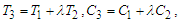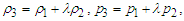are the viscosities of the waters; is the magnetic permittivity of the waters; are the kinematic viscosities of the waters. 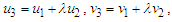River 3 is flowing with the combined flow variables of rivers 1 and 2 such that is a positive fraction.

The physical model of the merging/confluence problem is given in Fig. 1. Rivers 1 and 2 are flowing from different sources/mountains , merge at , and continued towards a standing water body . Upon this, the model is divided into two regions: the upstream region and downstream region with as the nodal or merging point. More so, for the geometric transition occurring between the merging rivers and the confluent river, the problem of the wall curvature effect exists. 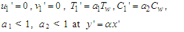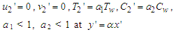To cater for this, we take a simple transition wherein the breadths of each of the rivers are assumed equal to half that of the confluent river, that is, and is non-dimensionally taken to be unity such that the merging angle is directly used (see [25]). Upon this, the boundaries become in the upstream and the downstream. Similarly, we assume the velocity of the merger-river to be .

Now, the boundaries conditions are:

(16)

(17)

(18)

(19)

for the upstream channels, and

(20)

(21)

for the downstream channel

Introducing the following non-dimensionalized quantities and stream functions:

(22)

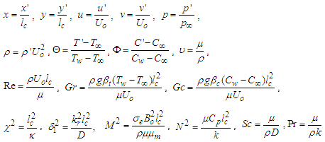
where Re is the Reynolds number; Gr is the Grashof number due to temperature difference; Gc is the Grashof number due to concentration difference. is the local Darcy number; M² is the Hartmann’s number; Pr is the Prandtl number; Sc is the Schmidt number; is the rate of a chemical reaction, and N² is the heat exchange parameter; is the scaled length, is the characteristic velocity, which is maximum at the centre and zero at the wall, and are concentration and temperature, respectively at which the river walls are maintained, and are the dimensionless temperature and concentration, and are dimensionless pressure, velocity in the x-axis, velocity in the y-axis and density, respectively; and are the dimensionless x- and y- axes, respectively, and

(23)

where is the stream function, and is the independent variable of the stream function, and

(24)

are the velocity components,

into equations (1) - (21), we have

(25)

(26)

(27)

(28)

with boundary conditions

(29)

(30)

and

(31)

(32)

(33)

(34)

with the boundary indications:

(35)

(36)

for the upstream channels, and

(37)

(38)

(39)

(40)

with the boundary conditions

(41)

(42)

for the downstream channel

where

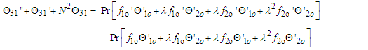
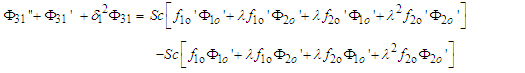
Equations (25) - (28), (32) - (34) and (37) - (40) are non-linear and coupled. Making them tractable, we seek for the perturbation series expansion solutions of the form:

(43)

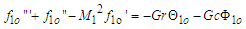
where represents the flow dependent variables, is the perturbation parameter. The choice of this parameter is based on the fact that, at the merging point, the interaction of the two rivers creates a sort of turbulence, implying an increase in the Reynolds number. will therefore give a very small value by which the problem is perturbed. It is interesting to note that the turbulence effects decay away some distances from the merging point and the flow normalizes.

Substituting equation (43) into equations (25) - (42) yields a set of equations that require some analysis. On the analysis of flow, we shall invoke the Kirchhoff Law of the flow of materials at the junction wherein the quantity of materials entering the junction is said to be equal to the total quantity of materials leaving the junction. Impliedly, the quantity of water/materials leaving Rivers 1and 2 for the junction is equal to the total quantity of water/materials in River 3. This tends to explain the fact that River 3 is the combined continuation of Rivers 1and 2. On this premise, we seek for approximate solutions to describe the problem. We choose the order zero equations as the equations describing the flow characteristics of Rivers 1 and 2 in the unperturbed state of flow, and the order one equations for River 3 as those describing the perturbed state of the flow downstream. Following this, the order one equations for the upstream flow and order zero equations for the downstream flow are played down. So, our working equations are reduced to

(44)

(45)

(46)

(47)

(48)

(49)

(50)

(51)

with the boundary conditions

(52)

(53)

(54)

(55)

for the zeroth order in the upstream,

and

(56)

(57)

(58)

(59)

with the boundary conditions

(60)

(61)

for the first order in the downstream

Expressing the order zero terms in equations (57) - (59) in terms , we get

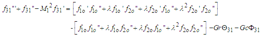(62)

(63)

(64)

The order zero equations describe the upstream flow, while the order one equations describe the downstream flow. More so, the presence of the order zero terms in the order one equations indicates the influence of the upstream on the downstream flow.

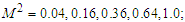
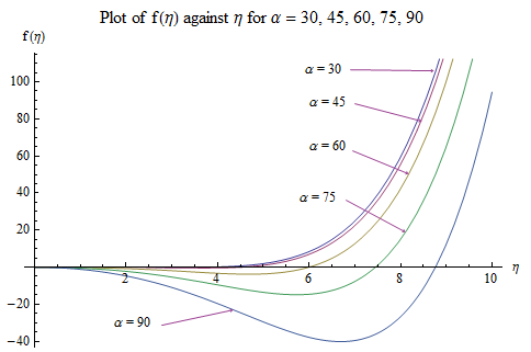
We investigate the effects of some hydro-dynamic parameters on the flow velocity structure of the merging two rivers, and their attendant implications on the transport of their bed-loads/sediments. The computations are carried out using the Mathematica 9 computational software. For constant values of and varied values of we obtained the graphs shown below. The figures show that the flow velocity is decreased by the increase in the magnetic field strength and merging angles but increases by the increase in the convective currents.

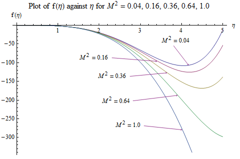Figure 2. Velocity ()-Magnetic field () profiles for

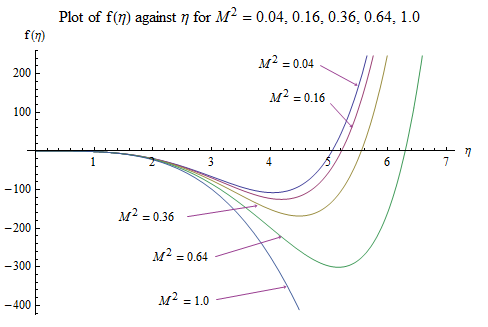Figure 3. Velocity ()-Magnetic field () profiles for

The effect of the magnetic field on the velocity is seen in Fig. 2 and Fig. 3. They show that the flow velocity decreases as the magnetic field strength increases. By the nature of the source rocks, the water of the river is alkaline or slightly acidic, and subsequently magnetically susceptible. Being alkaline, the water particles exist as charges. In the presence of the Earth magnetic field, which is due to the Earth rotation, they produce electric currents. The currents act on the magnetic field to produce a mechanical force, the Lorentz force. This force has the potency for freezing up flow velocities, and this accounts for what is seen in Fig. 2 and Fig. 3. More so, the magnitude of has some effects on the flow patterns; as can be seen in Fig. 2 and Fig. 3.

In a similar development, the porosity of the river channels has the same effects on the velocity as the magnetic field parameter.

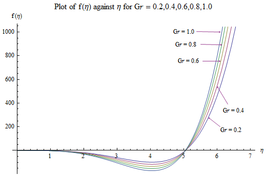
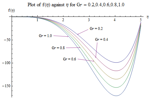Figure 4. Velocity ()-Grashof number () profiles for

Figure 5. Velocity ()-Grashof number () profiles for

The effect of convective currents (Grashof number) on the flow velocity is seen in Fig. 4 and Fig. 5. These figures depict that the flow velocity increases as the Grashof number increases. The temperature difference between the environment, which is due to the radiation from the sun, and the ambient temperature of the fluid in the presence of gravity, volumetric expansion coefficient due to temperature, viscous force and density effects create convective currents. The convective currents break the fluid particles from the grip of the fluid viscosity, thus making them buoyant and flow with ease. The ease of flow accounts for the increase in the velocity; as seen in Fig. 4 and Fig. 5. Similarly, the effects of the size of on the flow pattern are seen in Fig. 4 and Fig. 5. For the profiles tends to converge at for , the profiles converge at At this point, a flow separation, which may be due to an adverse flow condition, wherein is noticed. A short distance from this point, the profiles become distinct.

More so, the results here are applicable when the Grashof number which is due to the chemical concentration of the water is considered.

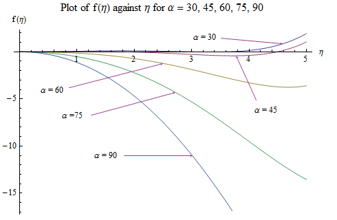Figure 6. Velocity ()-Confluence angle () profiles for

Figure 7. Velocity ()-Confluence angle () profiles for

Additionally, the effects of the confluence angle on the flow velocity are seen in Fig. 6 and Fig. 7. These figures show that the flow velocity decreases as the confluence angle increases. As the water of rivers 1 and 2 clashes into the merger, rotational and whirling/spinning motions are generated. This creates a sort of turbulence at the merging point. The rotation and spinning tend to reduce the motion in the axial direction, thus accounting for what is seen in Fig. 6 and Fig. 7. Significantly, the spinning motion creates scours at the merging point. Even so, the effects of the size of on the flow pattern, in the presence of the merging angle can be seen in Fig. 6 and Fig. 7.

The results show that, apart from the existing gradient/slope between the river and the source mountain, mass volume of the water, depth of the river, gravity, amidst others, hydrodynamic parameters affect the river flow, and subsequently affect the transport of the bed-loads/sediments. Usually, as the river flows downwards from the mountains, the particles eroded are carried along with them as bed-loads/sediments. The gradient effect highly enhances their transport in the upper and middle zones of the river, where velocities are high and moderate, respectively. The gradient effects subside or are decayed in the depositional zone. Naturally, the other factors and hydro-dynamic parameters effects take sway completely. Specifically, the decrease in the velocity by the increase in the magnetic field and porosity parameters and merging angle retard the transport of the bed-loads/sediments, thus causing early deposition of the materials and shallowing-up of the river. On the other hand, the increase in velocity through the increase in the convective currents and Reynolds number enhances the transport of the bed-loads/sediments, thus delaying the shallowing-up of the river in its course towards a standing water body.

3. Conclusions

A hydro-dynamic confluence flow model of two rivers is presented. The effects of some parameters: magnetic field strength, convective currents and merging angle on the flow velocity structure are investigated. The analysis of results shows that the increase in

• magnetic field decreases the velocity,

• Grashof number increases the velocity, and

• merging angle decreases the velocity.

The effects of these parameters on the flow have attendant implications on the transport of river bed-load/sediments.