Jay P. Narain
Retired, Worked at Lockheed-Martin Corp
Correspondence to: Jay P. Narain, Retired, Worked at Lockheed-Martin Corp.
| Email: |  |
Copyright © 2021 The Author(s). Published by Scientific & Academic Publishing.
This work is licensed under the Creative Commons Attribution International License (CC BY).
http://creativecommons.org/licenses/by/4.0/

Abstract
The solution of Blasius Equation with various numerical methods is reviewed. The Falkner-Skan equation is also solved with these methods. The application methods range from classical Euler, Runge-Kutta, to Artificial Intelligence Machine Learning methods. The code for each method is available for verification in python scripting language.
Keywords:
Blasius Equation, Falkner-Skan Equation, Fast and accurate solutions
Cite this paper: Jay P. Narain, Exploring Blasius and Falkner-Skan Equations with Python, American Journal of Fluid Dynamics, Vol. 11 No. 1, 2021, pp. 1-4. doi: 10.5923/j.ajfd.20211101.01.
1. Introduction
The solution of Blasius [1] and Falkner-Skan [2] equations for laminar boundary layer has been an interesting topic for over 100 years. There are overwhelming number of analytical and numerical methods to solve these equations. Presently numerical solution techniques from very basic Euler and RK4 integration and other initial value problem solvers with shooting method, boundary value problem with finite difference method, to the machine learning methods are discussed.
2. Discussions
The well-known Blasius [1] equation and boundary conditions are: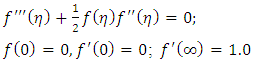 | (1) |
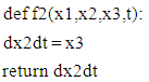
Where derivatives are with respect to eta, f being a function of 𝛈. The equation being non-linear cannot be solved by straightforward integration. This can be treated as both the initial value or the boundary value problem. For initial value problem, the general way to solve such an equation is to write it as a system of first order differential or partial differential equations as follows,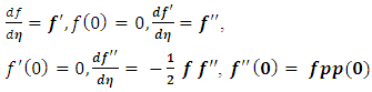 | (2) |
So, it boils down to simple three first order equations. Only problem is, we don’t have any idea what  A numerical scheme, known as shooting method, comes out handy. The solution of the set of equations are carried out for two initially guessed values of fpp(0). The objective is to achieve
  condition at the outer boundary. A secant method is used to get an estimate of updated value of fpp(0). The iterative procedure is carried out till outer boundary condition at
  . The outer boundary of
  is usually met at 𝛈 between 5 and 6.Euler Integration:This is classic integration scheme. For simplicity in coding and writing this paper, we will use following nomenclature,
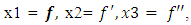 and t = 𝛈. The range of t, comprised of N points, is divided into equally spaced step size dt.
 | (3) |
 | (4) |
 | (5) |
Usually, a simple code in any language will give a converged solution in 5 to 6 iteration. The magic value of fpp(0) or x3(0) will appear as 0.332….. You will find many numbers after this basic value in literature. I have enclosed all the software on my website http://www/angelfire.com/co2/jpnarain/Euler_blausius_upd.py. This file contains the Blasius equation solver. Runge-Kutta4 Integration scheme:This scheme was developed over 100 years ago and has been one of the most accurate integration methods. This method is 4th order accurate compared to first order accuracy of Euler scheme. It is as fast as Euler method and as accurate as any higher order schemes for Blasius equation. The solution procedure is basically splitting the Blasius equation in three first order equation and use shooting method to get converged solution. Note, the method of integration involves different steps than Euler method. The outline for the method is,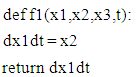 | (6) |
 | (7) |
 | (8) |
Integrate in the range of given t with following RK4 procedure. Remember we are solving simultaneous equations.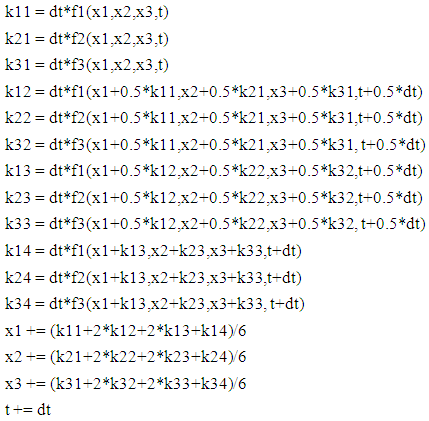 | (9) |
The Rk_blasius_upd.py shows the details of entire scheme.All the above and following Blasius equation solvers give the following nice plot: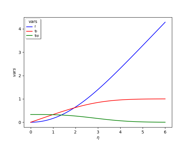 | Figure 1. Solution of Blasius equation by various methods |
Here are some public domain box solvers used for Blasius equation:1. Pycse [5] boundary value problem solver bvp. Works nicely and gives similar solution. Refer to pycse_blasius_bvp_upd.py code. This solver is little unstable for more complex equation, such as Falker-Skan [2] equation. Their bvp_nl works better and is similar to their finite difference approach discussed in following section 3.2. Octave [6] using lsode numerical scheme. Refer to files df1.m and df2.m to run Octave interactive setup. This is an initial value problem solver.3. A finite difference approach using scipy.optimize [5] fsolve solver. This is a very robust and reliable scheme. There is no shooting method involved and solutions are very accurate even in Falkne-Skan [2] favorable and adverse pressure gradient flows. It does not have any convergence problem with higher eta regions. It is simple to use and my most recommended method. Refer to file scipy_blasius_fds.py code.4. The artificial intelligence using machine learning has also caught up with the Blasius equation solution. The code enclosed here is from the creator of pycse group [5]. The concept of regression is used to update weight and bias while minimizing the equation function with boundary condition. This is also a non- shooting method. However the iterations used to minimize the function takes longer run time (140 s). Refer to mlBlas_Fs.py code.Note: There are couple of important variables in boundary layer theory, namely displacement thickness and momentum thickness. The displacement thickness is described as,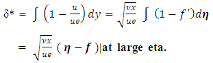 | (10) |
This is an exact solution. The numerical solution shows that  is constant after a value of
  = 4.99. This value is 1.7208.
 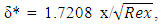 | (11) |
where Rex is the local Reynold’s number.Similarly, the momentum thickness is defined as: 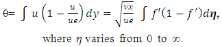 | (12) |
This has an exact solution of  | (13) |
Although these parameters can be evaluated as additional equations in Euler and RK4 schemes, it is nice to know that they have an exact solution.Falkner-Skan boundary layer equation [2]:The derivation of this similarity equation can be found in text books and on Wikipedia. It is similar to Blasius equation with additional terms to account for flow past wedge of angle πβ. The equation is: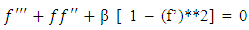 | (14) |
With boundary conditions: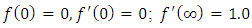 | (15) |
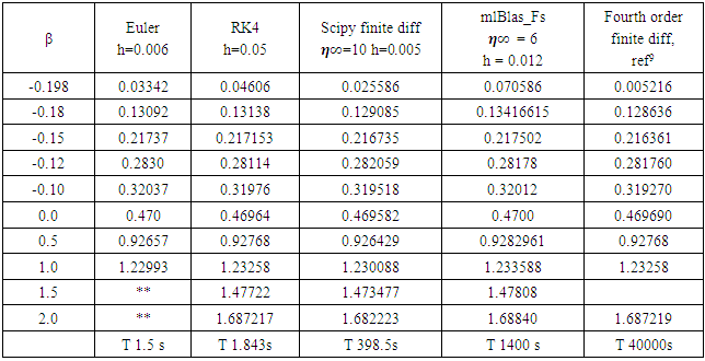
For β = 1, the problem is of flow impinging on a vertical plate, known as Hiemenz [3] flow. Here β < 0, corresponds to adverse pressure gradient (often resulting in boundary layer separation) while β > 0 represents a favorable pressure gradient. β = 0 corresponds to a modified form of Blasius equation. Douglas Hartree4 showed that physical solution to the Falkner-Skan equation exist only in range -0.198838 < β < 4/3. Our numerical solutions can reach β = 2. The stable method can go even higher, though these solutions are unrealistic.The solution procedure by various numerical schemes is similar to that of Blasius equation. The only difference in being the equation for f’’’ and presence of β. Apart from integration of simultaneous first order equations, I found subsequent integration for different β very useful as it alleviates guesswork for estimating f’’(0). The python lists were helpful in doing that. The following table 1. shows the value of f’’(0) for various methods and β.The method of minimizing the loss function based on the equation and boundary conditions, as described in the method of section 4, can be used to solve the Falkner-Skan equation for various β. Rackauckas8 has shown the theoretical background for solving the ODEs with Neural Networks which he describes as The Physics-Informed Neural Network. He solves a first order and a second order ode with a method similar to that described in section 4. After studying this article, any order ode can be solved with this scheme with confidence.Carlos Deque-Daza, Duncan Lockerby and Carlos Galeano [9] also solved Falkner-Skan equation using fourth order finite difference scheme. This should be considered as the most accurate solution. However, the other schemes give similar results, as shown in Table 1, with faster run times and similar accuracy except in near separation solution at β = -0.198.Table 1. The f’’’(0) for various β and various methods. The solution for ** exist, but f’’(0) has to be prescribed
 |
| |
|
The time shown will vary on your computer system. I used a 8GB, Intel i7 processor. The results are very similar for all the methods. Only solution from scipy finite difference method [5] is shown below 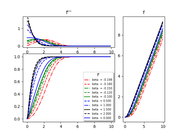 | Figure 2. Velocity f’ profile, Stream function f profile and Velocity gradient f’’ profile for various wedge angles (β) |
Various programs to solve this problem are posted on my website http://www.angelfire.com/co2/jpnarain/.Note: All the calculations were done in Python 3.6.2. As Python is open software and changes frequently, sometimes backward compatibility is not guaranteed. At present Python is at version 3.90. To make life easier, I will recommend using version 3.6.2.to 3.6.8. If you see error about some libraries not found, keep on downloading them from their ( .org ) websites. If you have never used Python, don’t worry, learning it is a piece of cake if you know any programming language.
3. Conclusions
I have briefly described the solution procedure for Blasius and Falkner-Skan equations. The programs are included for detailed work. This is from my class lecture note and is intended to encourage students to learn basic methods and to keep abreast with the developing technology.
References
| [1] | Blasius, H. , "Grenzschichten in Flüssigkeiten mit kleiner Reibung". Z. Angew. Math. Phys. 56: 1–37., 1908. |
| [2] | Falkner, V.M., and Skan, S.W., “Aero. Res. Coun. Rep. and Mem. no 1314”, 1930. |
| [3] | Hiemenz, Karl., “Die Grenzschicht an einem in den gleichförmigen Flüssigkeitsstrom eingetauchten geraden Kreiszylinder. Diss”. 1911. |
| [4] | Hartree, D. R., “Numerical Analysis. Oxford University Press.”, 1952. |
| [5] | John Kitchin, “pycse-Python3 Computations in Science and Engineering”, jkitchin@andrew.cmn.edu, 2018. |
| [6] | John W. Eaton, “GNU Octave, gnu.org/software/octave”, 1996-2020. |
| [7] | Pauli Virtanen, Ralf Gommers, Travis E. Oliphant, Matt Haberland, Tyler Reddy, David Cournapeau, Evgeni Burovski, Pearu Peterson, Warren Weckesser, Jonathan Bright, Stéfan J. van der Walt, Matthew Brett, Joshua Wilson, K. Jarrod Millman, Nikolay Mayorov, Andrew R. J. Nelson, Eric Jones, Robert Kern, Eric Larson, CJ Carey, İlhan Polat, Yu Feng, Eric W. Moore, Jake VanderPlas, Denis Laxalde, Josef Perktold, Robert Cimrman, Ian Henriksen, E.A. Quintero, Charles R Harris, Anne M. Archibald, Antônio H. Ribeiro, Fabian Pedregosa, Paul van Mulbregt, and SciPy 1.0 Contributors. (2020) SciPy 1.0: Fundamental Algorithms for Scientific Computing in Python. Nature Methods, 17(3), 261-272. |
| [8] | Chris Rackauckas, “Introduction to Scientific Machine Learning through Physics-Informed Neural Network, https://mitmath.github.io/18337/lecture3/sciml.jmd, 2020. |
| [9] | Carlos Deque-Daza, Duncan Lockerby and Carlos Galeano, “ Num sol of the Falkner-Skan equation using third order and high order compact finite- difference schemes”, J. of Braz. Soc. Of Mech. Eng., 2011. |

 Abstract
 Reference
 Full-Text PDF
 Full-text HTML