1. Introduction

Anony lake is a salted lake located in south of Am-boasary-Atsimo, in the south-eastern part of Madagascar in the coordinates: 46°29’E of longitude and 25°8’S of latitude. It can witness miscellaneous marine phenomena in the southern basin of the Indian Ocean since the coastline is in direct contact with this part of the ocean (figure 1).

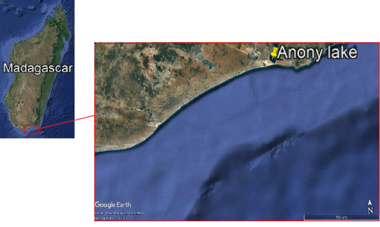Figure 1. Geographical position of Anony lake

Several researchers have long discovered the potential of this area in terms of fishing (Henneveux, 2010; Lamarque, 1957; G. Lasserre, 1979).

This leads us to look out for a merely scientific argument. More specifically, we suggest that the dynamic explanation of the substantial fish production is an upwelling phenomenon occurring permanently in this area.

Abundance in term of fisheries has always been scientifically related to upwelling, or technically, a phenomenon of rising seawater from depth. A large number of works has proven this argument in many region of the world, such as in Senegal (Siny Ndoye, 2017), in Peru (Vincent E. et al., 2005), in the Ivory Coast (Y Soro et al., 2009), in Guajira (Andrade & Barton, 2004). Hence, Echevin et al. in the study of upwelling in Peru, Chenillat in the study of upwelling in California (F. Chenillat, 2012), and all those above cited papers deal with Eastern Boundary Upwelling System commonly called EBUS.

Upwelling is a phenomenon that occurs in the open ocean and along coastlines: it is a process in which deep and cold water rises towards the surface. It is the result of the blow of winds across the ocean surface combined with the rotation of the earth. It causes the water to be pushed away and then water rises up from beneath the surface to replace the water that have been pushed away. The water that “wells up” from below is typically cold, dense and nutrient-rich. These nutrients “fertilize” surface waters, meaning that these surface waters often have high biological productivity. Therefore, good fishing grounds typically are found where upwelling is common.

G. David et al. (2006) in their review and study of oceanic current in the Indian ocean basin noted that the southeastern part of Madagascar can be biologically rich in nutrient because alongshore upwelling may exist there. That review is based on an older research lead by Piton and Magnier in 1975 in their study of hydrological circulation between Madagascar and the equator. Otherwise, in more current findings revealed that the East Madagascar Current or EMC force the upwelling in this area (Ramanantsoa et al., 2017).

Those background lead us to implement a numerical model in order to examine the characteristic of ocean circulation in this area. We simulate the ocean circulation in the seawater around Anony lake by using the ROMS (Regional Oceanic Modelling System) model.

The research in this paper is primarily focused on studying the movement of seawater particles in the study area through zonal, meridian and especially vertical velocities. The principle is to analyse the path of each water particle, whether or not they rise and tend to reach the shoreline. Knowing the behaviour of these parameters will provide us enough information about the possible existence of upwelling in the study area.

2. Methodology – ROMS Model Implementation

2.1. Dynamical Aspect and Mechanism

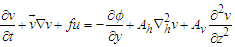
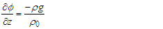
Due to the rotation of the earth, winds tend to turn right in the northern hemisphere and left in the southern hemisphere, technically known as the Coriolis effect. It is as a big part responsible of the upwelling in the coastal region.

According to the fundamental principle of dynamics, the motion of an elementary volume of fluid results from the balance of forces exerted on it. Through the Navier-Stokes equations, oceanic flows respond to this principle, while including the rotation of the earth. A major force in the ocean results from pressure variations around a fluid volume. The pressure depends on the density. And this can be inferred from salinity and temperature through a state relationship.

Thus, ocean modelling obeys to a system of 7 equations within 7 unknown parameters. Those equations, often called primitive equations, model a particle of sea water in motion. They contain the equation of motion (1,2), the hydrostatic equation (3), the equation of continuity (4), the equation of salt and heat (5,6), and the equation of State of the sea water (7).

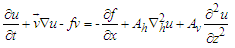(1)

(2)

(3)

(4)

(5)

(6)

(7)

Where are the components of the ocean velocity, f the Coriolis parameter, respectively the horizontal and vertical components of the viscosity and diffusivity coefficient, the density of the seawater, the reference density, g the gravity acceleration, S the salinity of the seawater, T the temperature of the seawater, the reference salinity and the reference temperature.

2.2. Numerical Methods and Scheme

ROMS is a numerical model which can run transient simulation for solving geophysical fluid mechanics equations in accordance with Boussinesq-approximation, hydrostatic approximation and incompressibility hypothesis. One of the major advantage of ROMS is that it can perform a discretization both on coastal areas and on terrain with very varied bathymetry. (P. Penven et al., 2010)

For solving the above primitive equations with upwelling configuration, given the indeterminacy of the turbulent flow terms, the system of equations requires the addition of so-called "closing" equations. So, horizontal isotropic turbulence and K-profil parametrization scheme (Large et al., 1994) have been adopted with Laplacian Horizontal mixing of momentum scheme.

The horizontal discretization of ROMS model implemented here adopt a traditional, centered, second-order finite-difference approximation with the Arakawa C-grid where the flow points are calculated in the faces of the mesh (Arakawa and Lamb, 1977). For vertical discretization, a second-order finite-difference approximation is also used but with a σ vertical grid type so as to get a better estimation of the topography.

Time-stepping use a split-explicit algorithm and divide the calculation into two modes: barotropic mode and baroclinic mode. Barotropic mode calculation is done between two time-step of the baroclinic mode.

2.3. Model Implementation

Using the ocean modelling process of ROMS model, we simulate the ocean motion that may carry out velocity output.

We took a study area along the geographical coordinates: 25°S-27°S of latitude and 45°E-47°E. In the simulation, this part of ocean is divided into 59 meridional grids, 44 zonal grids, and 32 levels.

The data used for the model include coastline and bathymetry database, lateral and surface forcing database, and climatology database. Those are mostly derived from satellite and in situ records as follow:

- GSHHS or Global Self-consistent, Hierarchical, High-resolution Shoreline Database which is a high-resolution shoreline dataset. (source: https://www.ngdc.noaa.gov/mgg/shorelines/gshhs.html).

- ETOPO2 for bathymetry, a 2-minute gridded global relief data (source: www.ngdc.noaa/mgg/global/etopo2).

- The Atlas of Surface Marine Data (ICOADS) for climatological data. It is monthly climatology (0.5 and 1° resolution) of air-sea parameters derived from individual observations (source: www.ncdc.noaa.gov/oa/climate/coads).

- The World Ocean Atlas 2009 (WOA) for forcing, a monthly climatology (1° resolution, 33 vertical levels) of in-situ ocean parameters derived from individual observations (source: www.nodc.noaa.gov/OC5/indprod.html).

3. Simulations of the Ocean Velocity

Upwelling system can be justified within the characteristics of the sea water dynamics, or its physical aspect (temperature and salinity, density, …). In this paper, we concentrate our study in the dynamics of the sea water represented by the ocean velocity. If sea water rises and moves to the coastal region, it means that the motion is under the lead of positive vertical velocity w, and the vector of horizontal velocity (combination of meridional v, and zonal u components) tend to veer to the coastlines.

The model output gives information about the average of each day of simulation. Each day is represented in a time index so that at the end of the simulation, the results contains 30 time indexes or 30 days.

The optimal iteration length according to the number of grids and the bathymetry is conforming to a criterion called CFL or Courant-Friedrichs-Levy (Katherine S., 2016):

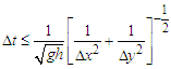(8)

To make sure of the significance of the model according to the grid resolution and time stepping, the courant number C must be less than 1. Consequently, the implemented model is done for 30 days’ duration containing 1080 iterations per day, giving a courant number equal to 0.46.

3.1. Horizontal Component of the Ocean Velocity

Firstly, it is important to analyse the horizontal view of the velocity to detect the direction of the horizontal velocity, and the value of vertical velocity. Vertical velocity is positive when seawater rise up and negative when the seawater drops down.

In horizontal view, the ocean velocity tends to point in the coastlines. That argument is permanently true during all days of the simulation but the velocity is high around the 29th day (figure 2). Even if in some minor regions the vertical velocity is negative, we can see that in almost all the region of the study area, it shows positive value.

We can clearly see the shape of the horizontal vector of the velocity tending to veer in the coast near Anony lake (around 46° 28’. So, in addition to its ascension, the seawater moves to the shoreline.

This figure can already be a part of proof that upwelling exists in the study area because it shows strong and positive value of vertical velocity combined with suitable direction of horizontal velocity.

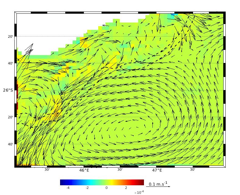Figure 2. Ocean velocity around Anony lake in the 29th day of simulation (vectors represent horizontal velocity; colors represent vertical velocity)

3.2. Vertical Profile of the Ocean Velocity

A profile view is taken in a transect (see figure 4) from a point A (of coordinates 46.43°E; 25.21°S) to a point B (of coordinates 46.45°E; 25.83°S) having about 60km of distance (figure 3).

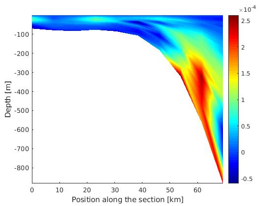Figure 3. Vertical ocean velocity along AB section, day 29

Positive vertical velocity manifests the ocean vertical motion in the observed section. We can detect a value of vertical velocity that rises the sea water from the bottom up to 200m depth at the day 29 of simulation.

3.3. Vertical Profile of the Velocity in a Specific Point around Anony Lake

Taking a point named P (with the coordinates: 46.39 °E of longitude, 25.18 °S of latitude, see figure 4) in the study area nearby the coastline around Anony lake, the vertical component of the corresponding velocity is given in figure 5.

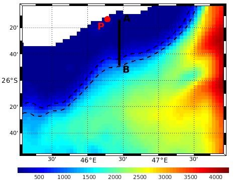Figure 4. Geographical location of the transect AB and the point P

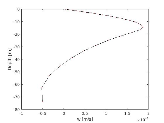Figure 5. Vertical profile of the velocity at the point P

We can find the highest value of w at 15 m depth of the ocean while the minimum value can be negative and found at the bottom of the ocean. From 40 m to 15 m depth, velocity is rising so as to reach the highest value near 2×10^-4 m/s. This figure also proves that in this ocean layer and moving to the surface, seawater particles are rising.

The time series given below (figure 6) show the evolution at 15 m depth of the vertical velocity in the point P during all the days of simulation.

We can observe a rising velocity as a function of time until the day around 16 and 17. The vertical component of the ocean velocity can reach 2.3×10^-4 m.s^-1 at 15 m depth.

It’s a high a positive velocity that make a reliable argument on the existence of upwelling in the study area. We can confirm the hypothesis that ocean “wells” from the bottom to the top with the optimal motion around the day 16.

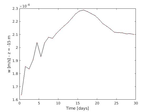Figure 6. Time series of the velocity at the point (46.39 °E; 25.18 °S)

4. Conclusions

The study of the ocean velocity can conduct to know where a moving particle can be in a given time. That was the main objective of this paper: to test whether ocean around the Anony lake “wells” or not.

The ROMS model implemented in this research is satisfying for it performs good calculation and optimal length of iteration is actually in accordance with grid resolution.

Values and directions of the velocity components are suitable for proving the existence of upwelling in the study area. Strong and positive values of vertical velocity have been detected in addition with horizontal velocity vector pointing in the direction of the coastline. There are some days around the day 16 of simulation where vertical velocity is positive and optimal in the chosen point. It can be translated as an upwelling period in that area.

Being previously mentioned by other authors (Ramanantsoa et al., 2017), the existence of upwelling phenomenon in the sea around Anony lake is confirmed by the findings of our current research. Anyway, in subsequent works, some parameters such as temperature and salinity may be included to better understand the upwelling in the study area.