1. Introduction

Swirling jets are commonly encountered in engineering applications, e.g., combustion chambers, premixed burners, mixing tanks, noise reducers, cooling systems, jet pumps, and turbomachines. Such swirling jets, single or coaxial, are often produced by superimposing a tangential velocity, called swirl velocity, on the axially directed flow issuing through the nozzle to enhance the rate at which it spreads into and entrains from its surroundings. A single swirling jet is desired for dilution and mixing at small distances from the nozzle while the coaxial jets for longer distances. Coaxial swirling jets form as fluids are issued through two concentric nozzles with either the inner or the outer jet swirling. In most of the applications, outer swirling coaxial jets are used because inner swirling coaxial jets develop like a single swirl jet as the inner swirl inhibits the penetration of outer flow towards its axis [1]. Coaxial jets develop through three successive regions as in Fig. 1, namely the initial region, intermediate region, and self-similar region. The initial region terminates with the disappearance of the outer potential core, the intermediate region terminates with the disappearance of the inner potential core, and the self-similar region initiates by the appearance of self-similar profiles of the flow properties. The initial and intermediate regions together are also known as the developing region and the self-similar region as the developed region [2].

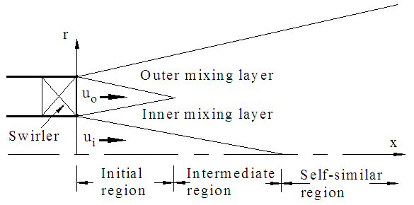Figure 1. Schematic of the coaxial outer swirling jets

Experiments [3,4] on coaxial jets show that the outer to inner jet velocity ratio (α) is the most important parameter in determining its mixing and flow properties in the developing region. Ko and Au [5] observed in the initial region of coaxial jets with small velocity ratio that the outer stream acts mainly as a coflowing stream which does not modify substantially the inner jet dynamics. Mergheni et al. [6] demonstrated experimentally that the coaxial jets with velocity ratio higher than unity develop faster and enhance mixing between the two streams by its ability to destabilize the flow. Ribeiro and Whitelaw [7] performed an experiment on coaxial jets with and without swirling. They showed that swirling coaxial jet develops at a faster rate in comparison to its counterpart. Furthermore, non-swirling coaxial jets approach the self-similar state in a smaller distance than a single round jet due to the interfacial interaction between the two jets.

Dahm et al. [8] carried out comprehensive flow visualizations in the developing region of coaxial jets. They conclude that a wide variety of dramatically differing vortex patterns result in very different interaction dynamics which may depend both on the velocity ratio and the velocity of two coaxial streams. Balarac and Metais [9] studied the near-field behavior of coaxial jets through direct numerical simulation. They found the jets to exhibit a reverse flow region in their inner part called recirculation bubble for α exceeds a critical value, and a pinch-off phenomenon near their inlet for high enough value of α.

A low swirling coaxial jet is known to produce a highly inhomogeneous scalar field at all downstream distances [10]. Present research is intended to study the coaxial jets numerically to ascertain the pattern of stratification that the swirling outer jet produces with the inner jet fluids at low swirl ratio. It is noteworthy that the author is not aware of any publication dealing with the pattern of such stratification of coaxial jets.

2. Governing Equations

The transport equation governing the steady state turbulent flow in generic form is

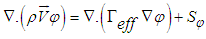(1)

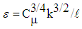
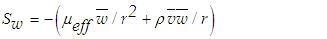
where is the density of the fluid, the velocity vector, the transport variable, the effective diffusivity and the source term. Here the variable represents the mean velocities the turbulent kinetic energy k and its dissipation rate ε, the mean concentration of species and the fluctuating concentration ξ. The term in full form for two-dimensional swirling flow in co-ordinates appears as

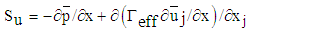(2)

(3)

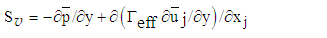(4)

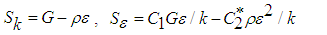(5)

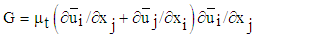(6)

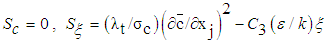(7)

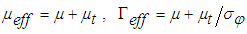
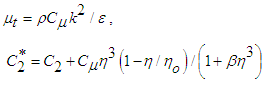
where , , equals the molecular viscosity, the eddy viscosity, the turbulent Prandtl number and the turbulent mass diffusivity which is assumed equal to .

2.1. Turbulence Closure

The commonly known feature of the re-normalization group (RNG) model that is the ability to capture the swirling flow and the findings of the researcher have encouraged its use in the present simulation of outer swirling coaxial jets. Marzouk and Huckaby [11] performed numerical simulations of coaxial particle-laden outer swirling air flow in a vertical circular pipe using three versions of the k-ε turbulence models: standard, RNG and realizable. Comparison with the experiment shows that the RNG model predicts the axial mean velocity quite satisfactorily than other versions of the model. For RNG k-ε model

(8)

(9)

where the closure coefficients Cμ =0.0845, σ_v=σ_w=σ_u=σ_c=1, σ_k=σε=0.7194, C₁=1.42 and C₂=1.68, η_o=4.38, C₃=1.786 and β=0.012.

2.2. Boundary Conditions

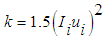
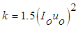
Coaxial plane jets have the following initial and boundary conditions. At the inflow for the inner jet , , , , and for the outer jet , , , and on the radial plane where u_i and u_o are the uniform velocities, I_i=3% and I_o=1.5% are the turbulence intensities, the turbulence length scale (assumed as 20% of outer jet diameter) and c_i the uniform species concentration. At the free stream , at the outflow and at the axis of symmetry except . The outer swirling coaxial jets have the same initial and boundary conditions along with the additional conditions at the inflow for the inner jet and for the outer jet and at the axis of symmetry . For both types of coaxial jets, with and without swirl, zero pressure is specified at all boundaries besides the axis of symmetry. Further, an external axial velocity of 3% of the inner jet velocity is imposed on the coaxial jet flow to provide stability to the numerical scheme.

3. Numerical Procedure

A computational fluid dynamics (CFD) code is developed based on Semi-Implicit Method for Pressure-Linked Equations (SIMPLE) algorithm [12] for solving the general transport Eq. (1). The convective and diffusive terms of the transport equation are discretized using the second-order upwind difference scheme and the second-order central difference scheme, respectively. Discretized transport equations for are solved iteratively using the line by line tridiagonal matrix algorithm (TDMA) [13]. Three sweeps are sufficient for momentum, kinetic energy, and dissipation equations, also for mean and fluctuating concentrations equations but five sweeps are required for pressure correction equation. All the variables are weighted with the appropriate under-relaxation factor to stabilize the computer program. These relaxation factors are 0.7 for , and 0.3 for , and 0.5 for . The solutions are considered converged when the sum of normalized residuals of fall below 510^-6. The flow domain is constructed over 20d_i40d_i in r-and x-directions with the staggered grid that clusters axially near the jet exit and radially near the jet interfaces, and further apart with increasing distances in both directions as in Fig. 2 where d_i is the inner jet diameter.

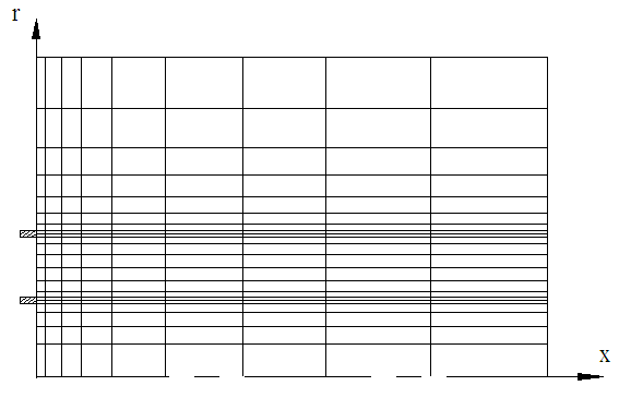Figure 2. Computational grids for the coaxial jets

3.1. Present CFD Code Validation

The developed CFD solver is validated with the experimental work of Sadr and Klewicki [14] on coaxial plane jets for the Reynolds number Re_i= 4.110⁴ based on the inner jet diameter and velocity. The maximum uncertainty estimate in their measured instantaneous velocity is about 0.2% u_i in the wake region of the inner jet wall at x/d_i=0.07. Code validation and grid convergence test for the present simulation are performed on coaxial plane jets for Re_i= 410⁴. The inner and outer jet diameters are d_i=0.04m and d_o=0.072m, and the inner and outer jet velocities are u_i=15m/s and u_o=0.18u_i.

A grid convergence test is carried out with the three grid sizes (ninj) termed coarse, medium and fine which are 141248, 151266 and 171302 where ni and nj are the numbers of grid points in r and x-directions. Figure 3 shows the radial profiles of the axial mean velocity at x/d_i=6 for the three grid sets. Grid refinement shows successful convergence with those three grid resolutions and the results presented in this paper are obtained using the fine mesh. Quantification of numerical uncertainty is made by using the guidelines in [15] as follows. The discretization uncertainty in the fine-grid solution for the axial mean velocity at x/d_i=6 and r/d_i=0.5 is calculated as 0.76% for a grid refinement factor of 1.22. The uncertainty in iteration convergence of the fine-grid solution for the same axial velocity over the radial plane at x/d_i=6 is determined as 0.002%. Further, the values of 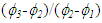for the same axial velocity are found positive that indicate a non-oscillatory convergence.

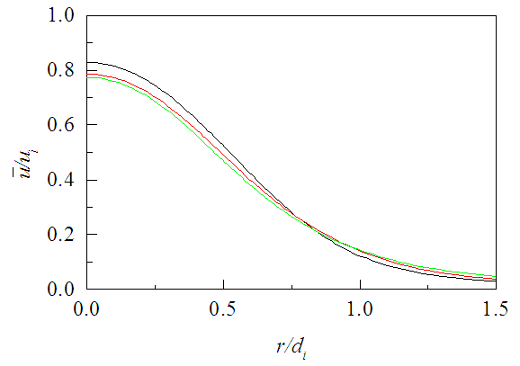Figure 3. Axial mean velocity profiles at x/di=6. Grid points

Comparison of the results in Figs. 4-5 exhibits that centerline axial velocity of the simulation decays faster compared with that of the experiment. This faster decay of the jet is known to be the limitation of RNG k-ε model like the standard k-ε model [16]. However, the profiles of normalized axial mean velocity are in good agreement with the experiment. The mean velocity profile at x/d_i=0.07 shows some difference which is due to that at x/d_i=0 the outer jet extends to r/d_i≤0.9 in the simulation and r/d_i≤1.25 in the experiment. Thus, the comparison shows that the present results are in good agreement with the experimental data and the in-house developed software gives satisfactory results.

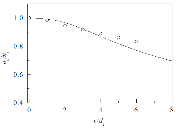Figure 4. Centerline velocity decay for α = 0.18. Line for simulation and symbol for Sadr and Klewicki [14]

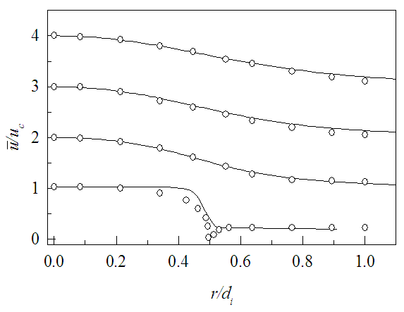Figure 5. Profiles of axial mean velocity for α = 0.18 at (from bottom) x/di=0.07, 2, 4 and 6. Ordinates are shifted by 0.5(x/di) units. Lines for present simulation and symbol for Sadr and Klewicki [14]

4. Results and Discussion

Numerical simulation of outer swirling coaxial jets is performed for the swirl ratios 0.2, 0.4 and 0.8, with a velocity ratio of 0.3. This simulation of coaxial jets is made by assuming an incompressible air flow of mach number 0.04 for the largest jet velocity at inflow. The swirl of a flow is the measure of its rotation expressed by the ratio of the axial flux of angular momentum to the axial flux of axial momentum of the coaxial streams [17], called the swirl number, as

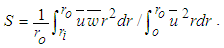(10)

Equation (10) provides the range of swirl number as 0.03≤ S ≤ 0.11 corresponding to the swirl ratio 0.2≤ SR ≤ 0.8 for SR=w_o/u_o. Extracted results from the present simulation of swirling coaxial jets are presented in this section as the radial and axial profiles of mean velocity, mean vorticity, mean and fluctuating concentrations, and helicity for a fixed velocity ratio (α=u_o/u_i) with different swirl ratios.

4.1. Mean Velocity

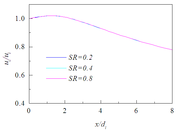
The profiles of axial mean velocity against r/d_i are plotted in Fig. 6 for the three axial positions x/d_i=0.5, 2, 4. The velocity profile at the jet origin (x/d_i=0) is discontinuous because of the presence of nozzle walls. These walls create a double-humped velocity profile as observed at x/d_i=0.5 which disappears with increasing downstream distance at x/d_i ≥ 2, and results in velocity profiles nearly same as that of a single circular jet. The displayed velocity profiles at each axial location contain three profiles with SR=0.2, 0.4 and 0.8 showing no discernible effect of swirl ratio (this happens to the axial and radial mean velocity, mean vorticity, mean and fluctuating concentration profiles in Figs. 6-8 and Figs. 12-16). This is because the swirl number in the present simulation (S≤0.16) is below the point of classical instabilities, e.g., vortex breakdown, to occur [18]. Mean axial velocity along the jet centerline is shown in Fig. 7 against the downstream distance x for different SR. There the jet centerline velocity is seen to be accelerated due to the momentum gain from the outer swirling jet. The centerline velocity is also seen to be independent of the swirl ratio in the downstream because of the small swirl number in the present simulation which cannot affect the inner jet dynamics significantly under a fixed small velocity ratio.

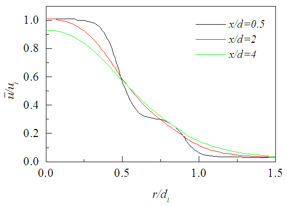Figure 6. Axial mean velocity profiles at different axial locations for SR = 0.2, 0.4, 0.8

Figure 7. Centerline mean velocity decay for different SR

Figure 8. Radial mean velocity profiles at different axial locations for SR = 0.2, 0.4, 0.8

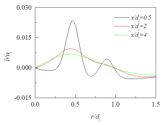
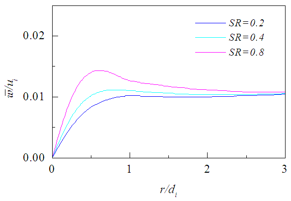
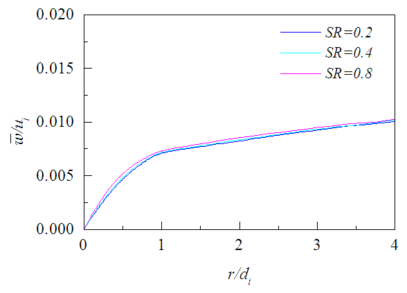
Radial mean velocity is shown in Fig. 8 against r/d_i for the three axial positions and three swirl ratios. This velocity profile evolves in the downstream similar to the axial velocity but requires a little longer downstream distance for the effects of nozzle walls to be washed out, because the radial velocity is weak to outweigh the effects rapidly. Figures 9-11 presents the tangential velocity against r/d_i for the same three axial positions and and swirl ratios. These velocity profiles are found to depend on the swirl ratio and quickly die down in the downstream compared to the axial velocity due to the momentum loss both to the surrounding and to the inner jet. Moreover, the profile of achieves a small constant value compared to the imposed external velocity after some radial distance.

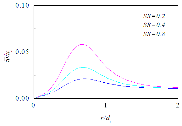Figure 9. Tangential mean velocity profiles at x/di = 0.5 for different SR

Figure 10. Tangential mean velocity profiles at x/di = 2 for different SR

Figure 11. Tangential mean velocity profiles at x/di = 4 for different SR

4.2. Mean Vorticity

Normalized mean vorticity Ωd_i/u_i is presented in Fig. 12 against r/d_i for the three axial positions where . The vorticity profile evolves in the downstream and the double-humped profile washed out at x/d_i>2, i.e., requires a little longer downstream distance compared to -velocity as its radial gradient constituting the vorticity is more sensitive to the presence of nozzle walls. As long as is constant, the figure shows that the vorticity profiles remain unaffected under the changing swirl ratio (this happens to all the properties presented here except the swirl velocity and helicity).

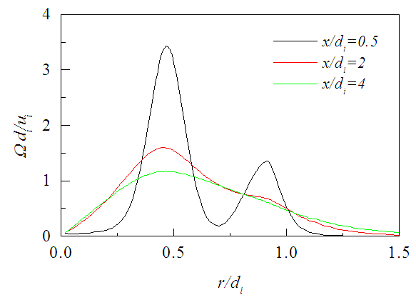Figure 12. Mean vorticity profiles at different axial locations for SR=0.2, 0.4, 0.8

4.3. Mean Concentration

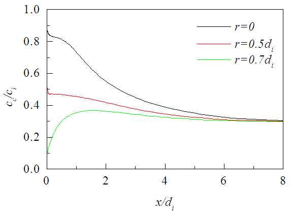
Figure 13 exhibits the normalized mean concentration that decreases radially due to the decaying velocity field and entrainment of ambient fluids. The concentration of the jet fluid is the largest on its centerline that dilutes in the downstream due to the vortex breakdown (if occur) in addition to the above factors. Figure 14 shows the axial variation of at different radial distances r=0 (center of the inner jet), r=0.5d_i (interface of the two jets) and r=0.7d_i (center of the annular space) and further shows that achieves a value of nearly 0.3 over the radial plane at x/d_i >8.

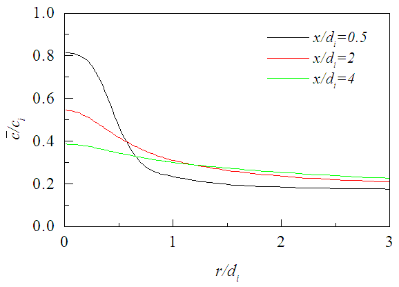Figure 13. Mean concentration profiles at different axial locations for SR=0.2, 0.4, 0.8

Figure 14. Centerline mean concentration for SR=0.2, 0.4, 0.8

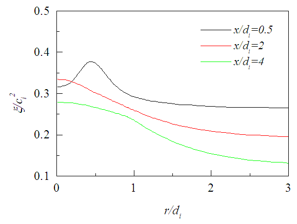
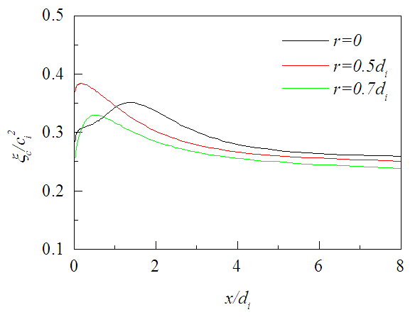
4.4. Fluctuating Concentration

The rms fluctuation of concentration ξ is displayed in Fig. 15 over different radial planes. The hump in the fluctuation profile at x/d_i ≤ 2 is the effect of nozzle walls. Figure 16 shows that rms fluctuation is not zero in the potential core of the jet rather increases corresponding to the increase in centerline velocity within the core region. The axial profiles of fluctuating concentration become constant at x/d_i>8 like the mean concentration but vary with the radial distances, although the increase or decrease of fluctuating concentration depends on the balance among the convection, diffusion, production, and dissipation of the rms fluctuations.

Figure 15. Fluctuating concentration profiles at different axial locations for SR=0.2, 0.4, 0.8

Figure 16. Fluctuating concentration at different radial distances for SR=0.2, 0.4, 0.8

4.5. Mean Helicity

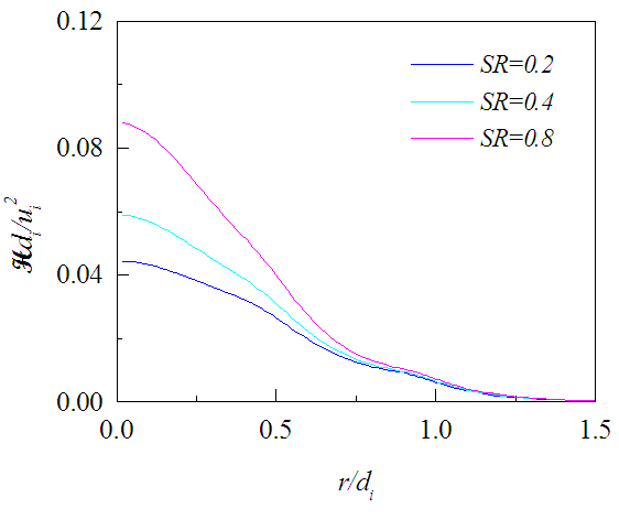
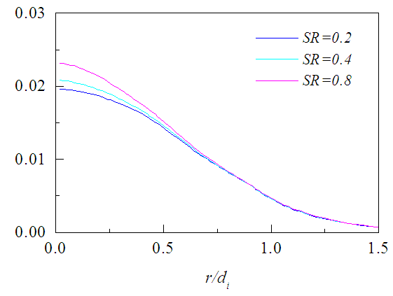
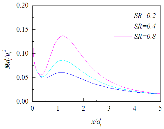
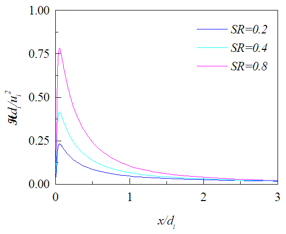
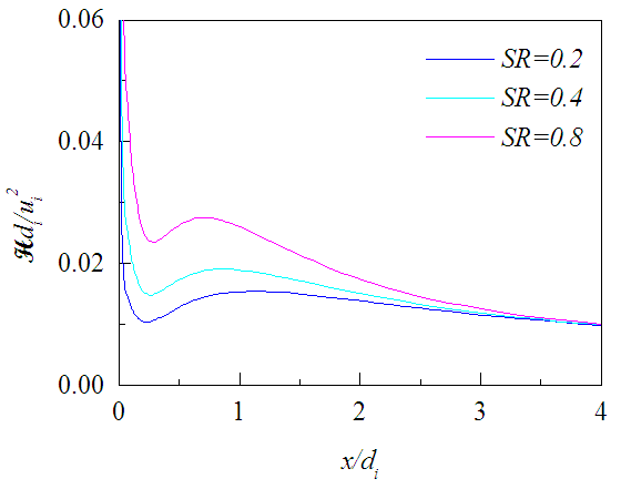
It is a scalar product of the velocity vector and the vorticity vector, mathematically written as , is shown in Figs. 17-19 against r/d_i for the three axial locations where it decreases radially outward except on the planes close to the jet exit. There the level of radial profiles of Hdi/u_i² are found to increase with the increasing swirl ratio due to the increase in tangential velocity and die down radially outward as quickly as the tangential velocity. Figures 20-22 exhibit the axial evolution of the helicity at three radial distances. The axial profiles show that Hdi/u_i² is much stronger at the interface of two jets compared to that at the center of the inner jet or annular space for all swirl ratios. Figure 20 also exhibits that helicity on the jet axis increases rapidly with the increasing proximity of the jet exit for x/d_i<0.5 which may be due to large radial variation of the swirl velocity.

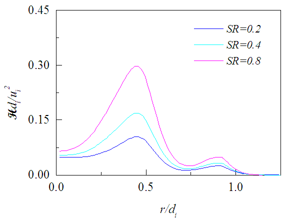Figure 17. Mean helicity profiles at x/di = 0.5 for different SR

Figure 18. Mean helicity profiles at x/di = 2 for different SR

Figure 19. Mean helicity profiles at x/di = 4 for different SR

Figure 20. Mean helicity profiles at r=0 for different SR

Figure 21. Mean helicity profiles at r = 0.5di for different SR

Figure 22. Mean helicity profiles at r = 0.7di for different SR

5. Conclusions

Numerical simulation of the coaxial jets for an incompressible flow of air with and without swirl has been performed. Turbulence closure for the equations governing the flow is achieved by using RNG k-ε model. Results from the simulation for swirl ratios 0.2, 0.4, 0.8 show that the mean flow structures, and mean and fluctuating concentrations remain unaffected against the change in swirl ratio except for the swirl velocity and mean helicity.

Axial profiles of the helicity at different radial distances show that low swirl causes small helicity. This small helicity induces low spiral motion to the jet fluids which may create large-scale structures. It seems encouraging for homogeneous charge compression ignition engine (assuming air-fuel in the inner jet and exhaust gas in the outer jet), as in recent times, the engine has become promising having the advantage of large-scale stratification of the premixed air-fuel mixture (homogeneous relevant to the chemical kinetics) by the exhaust gas recirculation [19].