1. Introduction

In the case of an actual voyage, ships rarely travel in head waves as they offer the highest added resistance and bow slamming. Common practice in ship hydrodynamics is to predict added resistance by simulating head wave cases and make assumptions for oblique wave cases basing on head wave results. Naturally, this method has limitations as different bow and stern shapes react differently to oblique waves. Furthermore, at high seas with large wave heights, the design of the ship hull above the water line becomes particularly important, which is mostly ignored in potential theory based simulations. In oblique waves, motion stability also acts differently and rudder action becomes important. Thus, oblique wave simulations are necessary to properly evaluate a hull form design and to get a realistic idea of its behavior during the actual voyage.

Application of Reynolds averaged Navier-Stokes (RaNS) equation based Computational Fluid Dynamics (CFD) solvers in predicting ship resistance and motion is nothing new in the field of ship hydrodynamics. RaNS solvers have reached a level of maturity in recent years following decades of development work by numerous researchers. Among recent contributions, in 2003, Orihara and Miyata [1] used a code named Wisdam-X that solved an overlapping grid system, using finite volume method, to solve ship motions in regular head waves and evaluated added resistance of a series of different bow-forms for a medium-speed tanker. Later in 2007, Carrica et al. [2] simulated surface ships in regular head waves, free to heave and pitch, using a solver named CFDShip-Iowa, which solved RaNS equation with the single-phase level set method. Castiglione et al. studied added resistance and response of high-speed Delft Catamaran in head wave and showed the peak motion is always at the resonance frequency, and the peak increases with increasing speed. Deng et al., Moctar et al. and Sadat-Hosseini et al. presented added resistance prediction results for KVLCC2 in head waves in Gothenburg 2010 workshop [3], for wave lengths 0.6L, 1.1L and 1.6L. The same cases were also simulated by Deng et al. [4] using ISISCFD, Moctar et al. by Open FOAM and Comet, and Sadat-Hosseini by CFDShip-Iowa. Visonneau et al. also conducted ship motion analysis using ISISCFD in 2010. The code was also validated by Guo et al. [4] for calculating added resistance of KVLCC2 in head waves. In 2013, Sadat-Hosseini et al. [5] further extended their initial work by showing added resistance prediction for KVLCC2 in short and long wave length cases with fixed and free surge motion. Kim et al. [6] also validated added resistance cases for KVLCC2 in 2013, using a RaNS code named WAVIS, developed by KRISO. Larsson et al. performed a comparative study of various CFD methods for KVLCC2, KCS and DTMB5415 ship models. In another study, Larsson et al. [3] concluded that the number of grid points used in CFD has an obvious effect on both motions and resistance results. A further comparison study of CFD methods to predict added resistance was performed by Soding et al., where he used potential flow Rankine Panel Method and experimental results, and concluded that predictions from CFD method are closer to experimental results in long wave region but less accurate in shorter waves. A detailed study of both steady and unsteady ship motions was also conducted by Simonsen et al. [7] in 2013, which compared experimental results for KCS model, with CFD predictions by CFDShip-Iowa and commercial code Star CCM+. He reported that the mean resistance was accurately predicted by CFD, however, the amplitude of resistance variation with time was under-predicted. Shen et al. [8] modified the open source CFD solver, OpenFOAM, to incorporate overset grid and performed maneuvering simulation for appended hull. Sigmund and el-Moctar [9] used COMET and modified OpenFOAM solver to perform added resistance simulations for four different hull types.

Although much work has been done on CFD simulations in head waves, research on added resistance prediction in oblique waves has been very limited so far. Among the recent works, McTaggart [10] performed oblique wave simulations for FFG 7 using both near and far field method and showed that near-field method produces better agreement with experimental data. Chan et al. [11] introduced a nonlinear time domain simulation method incorporating Euler equations of motion, to predict large amplitude motion of a Ro-Ro ship in regular oblique waves, both in intact and damaged conditions. The study showed good agreement with the measured data except in roll-resonance region, where non-linear effects are significant. Orihara [12] conducted RaNS simulations for an SR108 container ship in oblique regular and irregular waves and achieved good agreement with experimental data. However, he used a modified stern to avoid numerical instability. Jing and Zhu [13] used the time domain Rankine panel method to predict the motion of a container vessel in oblique waves, together with an artificial spring model to control sway and yaw motion, and an empirical method for roll damping. Whereas, Song et al. [14] applied the concept of the weakly nonlinear formulation to the 3D Rankine panel method in time domain approach to predict nonlinear motions and hull-grinder loads of a container ship in oblique waves. Wang et al. [15] used RaNS equation and kinematics equations of a rigid body to solve a moving grid, together with the sliding grid technique, to simulate the motion of surface combatant with heave, pitch, and roll free motion. He compared the results with that based on linear strip theory and found good agreement. Duan and Li [16] used a method combining Gerritsma and Beukelman (G & B) together with Salvesen-Tuck-Faltinsen (STF) and the DSG method. They used the method to calculate the added resistance profile for a wide range of wave lengths in oblique waves for a container and a tanker ship. Chuang and Steen [17] also used the STF strip theory to directly calculate speed loss of a tanker vessel due to oblique waves. More recently, in Tokyo 2015 workshop, some results for oblique wave simulation cases were presented for KCS model, and submission were also made by several research groups for validation. Recently, Rahaman et al. [18] used a commercial PF solver to provide oblique wave forces and motions for KCS, KVLCC2, and JBC model. Shigunov et al. [19] provided a comparative study for oblique wave simulations for DTC and KVLCC2 hull form using RANS and Panel method simulations, and compared the results with experimental data. However, the KVLCC2 results were for zero forward speed.

It is generally difficult to perform oblique wave experiments because of the limited width of water tanks, which does not allow sufficient run duration to reach steady oscillating motion. Recently constructed wave tank facilities do provide some solution to such limitations, however, they are very expensive. Although some potential flow-based methods can predict added resistance in oblique waves, their accuracy level is still limited due to the high non-linearity involved in such conditions. Potential theory based simulations being irrotational and non-viscous [20], have limitations regarding evaluation of viscous phenomenon prevailing at the stern part of the ship, which restricts their capability in differentiating design modifications at the stern part. In the case of RaNS solvers, generally in head wave cases, simulations are run assuming the symmetry of a ship (only half of the domain is simulated, either starboard or port side of the ship), with just heave and pitch free motion. However, for oblique waves, the full hull is to be simulated for getting roll, sway and yaw motions. Such simulations are both difficult and time-consuming to perform. Thus, oblique wave simulation results are very limited for RaNS solvers.

This paper contains simulation results for the KVLCC2 ship model, simulated with five degrees of freedom (DOF), in oblique wave conditions, for short wave length cases, using an in-house RaNS solver named SHIP_Motion. Predicted results are shown for added resistance coefficients, and response amplitude operators (RAOs) in heave and pitch, for three different bow heading angles. In order to improve confidence on results, first, head wave cases were validated, next, oblique wave simulations were performed, maintaining the same simulation conditions and mesh resolutions. For comparison, simulations were also performed in oblique waves using a commercial potential flow based solver named HydroSTAR. However, the paper simply presents a case study for ship behavior in oblique waves, and doesn’t attempt a validation study for the RaNS solver in predicting oblique wave results. Thus, only trends are discussed in the paper, and not the predicted values.

2. Computational Method

2.1. Mathematical Model of the Solver

The mathematical model of the solver is based on the model described by Orihara [12]. However, the solver code has received several contributions and revisions over the period. A brief description of the code is provided in this section. Further detail is available in the thesis of Islam [21].

The SHIP_Motion follows two sets of coordinate system, the body fixed (o-xyz) and the earth fixed (O-XYZ), defined in Cartesian coordinate system (Figure 1). In both coordinate systems, xy-plane is defined as the free surface and the Euler transformation is used to switch between coordinates.

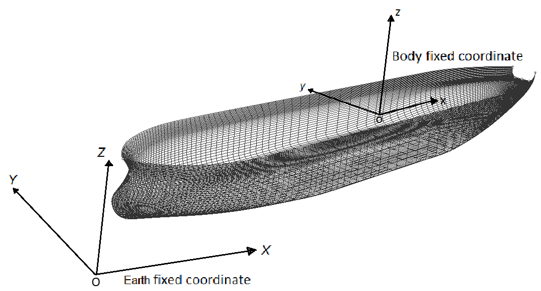Figure 1. Definition of coordinate system in SHIP_Motion

The governing equations are the RaNS equation and the continuity equation. The equations are expressed in integral form for a control volume Ωc and control surface Ωs as followed:

(1)

(2)

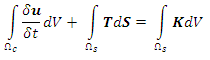
Where, is the time differentiation for the control volume, u is the fluid velocity vector, T is the fluid stress tensor, and K is the body-force vector accounting for the inertial effect due to the motion of the coordinate system. T is expressed as:

(3)

Where, I is the identity tensor, Re is the Reynolds number, is the gradient operator, (·)^T denotes the transpose operator, and is the piezo metric pressure excluding the hydrostatic pressure, which is defined as:

(4)

Where, p is the static pressure and Fr is the Froude number. The kinematic viscosity is evaluated by the turbulence model. The body force vector K is calculated as:

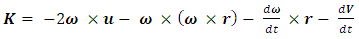(5)

Where, ω is the angular velocity of the body-fixed coordinate system, r is the relative position from origin-O, and V is the translation velocity vector of the ship in the directions of x, y and z Orihara [12].

For the spatial discretization, SHIP_Motion uses the Finite Volume Method (FVM). The kinematic condition for mass conservation is treated using the density-function method [22], [23]. Where, ρ_m is defined in the computational region as:

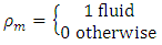In the control volume, including the free surface, the value of ρ_m is approximated by the fractional volume of the fluid that occupies the cell. Then the location of the free surface is defined as the iso-surface of ρ_m= 1/2. The time-dependent evolution of the density function is determined by solving the transport equation of ρ_m, which is written as:

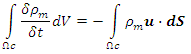(6)

Where, u is the fluid velocity. The right-hand side of the above equation is discretized using the QUICK scheme [3] and temporal discretization is the second-order Adams–Molton method.

The dynamic condition of the free surface is treated by extrapolating the velocity and the pressure above the free surface. The surface tension and external stress on the free surface are ignored, and the zero-stress condition is approximately satisfied on the free surface.

Incident waves are generated in a manner based on linear wave theory (Airy Wave Model). The generation of incident waves is approximated by giving the fluid velocity and wave height explicitly at the inflow boundary of the outer grid. The wave height and the fluid velocity due to the wave particle motion u_w are given in the earth-fixed coordinate system as follows:

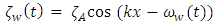(7)

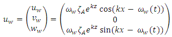(8)

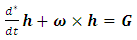
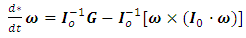
Where, is the wave amplitude, k = ω_w²/g, is the wave number, and ω_w is the angular frequency. Equation 7 is implemented by giving the values of the density function that the vertical location of the iso-surface of ρ_m = 0.5 coincides with the wave height given by equations.

On the ship body boundary, the no-slip condition is imposed for fluid velocity. To reduce the requirement for minimum grid spacing in the direction normal to the body surface, Spalding's universal wall function model is employed. The body-boundary condition for pressure is derived by incorporating the no-slip condition for the velocity into the RaNS equation (Eq. 1), and assuming that the inner product of the diffusion term and the normal vector to the body surface is zero. The gradient of the density function normal to the body surface is assumed to be zero. Except for the case of zero advance velocity, a uniform flow is given at the inflow boundary of the outer solution domain. At the outflow and side boundaries of the outer solution domain, the open-boundary condition is imposed for all the flow variables. At the center plane boundaries, symmetry condition is imposed for all the flow variables, when symmetry condition applies. At the inflow, outflow, and side boundaries of the inner solution domain, the Drichlet boundary conditions are obtained by interpolating the flow variables of the outer solution domain as described in the overlapping grid calculation.

The dynamic sub-grid scale (DSGS) turbulence model is applied for solving the outer mesh and the Bladwin-Lomax (BL) model [24] is used for solving turbulence in the inner mesh. Spalding’s universal model of the wall [25] is used as wall function to reduce mesh dependency for capturing the boundary layer, which allowed compromise in y+<1 criteria, where y+ is the non-dimensional boundary wall thickness.

Differencing for advection is done by the 3^rd order upwind scheme and the 2^nd order central difference is used for other discretization in space. The definition of the physical variables is in a staggered manner, that is, the pressure is defined at the cell or volume center and the velocity quantities in Cartesian coordinates are defined at face centers.

Temporal discretization is by the 2^nd order Adams-Bashforth explicit method. As for parallel computing, the OpenMP shared memory model is used [26].

A Marker and Cell (MAC) type pressure solution algorithm is employed. The pressure is obtained by solving the Poisson equations using the Successive Over Relaxation (SOR) method, and the velocity components are obtained by correcting the velocity predictor with the implicitly evaluated pressure.

In the solver, the ship motion is solved using the equations of ship motion. The equations for translational and rotational motion are as followed:

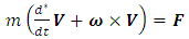(9)

(10)

Where, h is the angular momentum, m is the mass of ship, and is the time differencing for body-fixed numerical coordinate system.

The hydrodynamic force F and moment G are gained by integrating the fluid stress on the wetted surface of the ship. The acceleration of the ship in the body fixed coordinate system is obtained by solving the Eq. 9 for V.

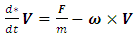(11)

The angular acceleration for rotating motion calculation is gained by substituting h = I_o∙ω, in the Eq.8.

(12)

Where, I_o^-1 is the inverse inertia tensor matrix.

Finally, linear (V) and angular (ω) velocities are calculated by integrating Eqs. 9 and 10 with respect to time. Then they are transformed from the body-fixed to the earth-fixed coordinate system and linear trajectory of the center of gravity (c.g.), and attitude of the ship is obtained by integration in the earth fixed domain.

For incorporating the surge motion, a numerical spring system is incorporated following experimental setups.

(13)

(14)

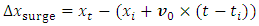
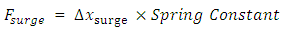
Here, is surge force, Δx_surge is surge displacement, x_t is ship's position at present time step, x_i is ship's position at the start of motion, v₀ is the initial ship velocity, t is the present time and t_i is the time at start the of motion. The surge force is added to the thrust force. For the simulation cases presented here, the surge spring constant was set at 0.01, for unit ship length.

In the overlapping grid system, the inner domain moves according to ship’s equation of motion and the outer domain represent free surface. Grid points located at the overlapping region exchange information through interpolation to update both the domains at every time step. For updating the flow process, prediction-correction method is used. First, hydrodynamic force and moment are predicted from flow solution at present time step. Next, ship’s linear and rotational velocity is computed, from which, body force is gained. Again, pressure and velocity of the flow field are calculated. The process is repeated again for corrected predictions. The process is shown in Figure 2.

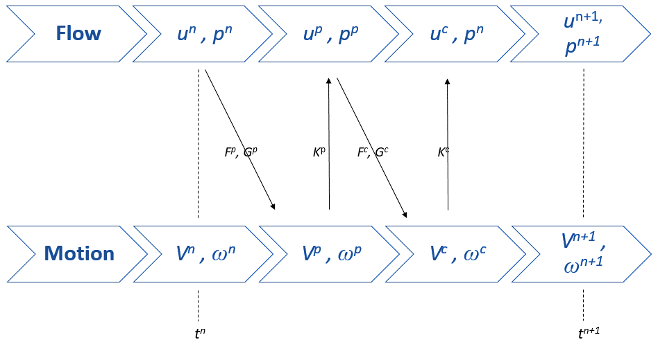Figure 2. Prediction-correction scheme for coupling ship motion and flow computation in the solver

2.2. Ship Model and Meshing

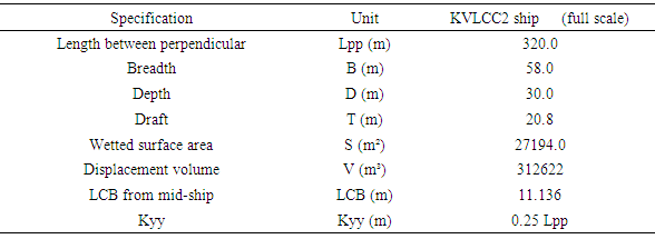
The ship model used in this research paper is the KRISO Very Large Crude Carrier 2 (KVLCC2) [27]. It is a tanker ship designed by MOERI (Maritime & Ocean Engineering Research Institute, formerly named KRISO) for research purpose. Table 1 provides the specifications of the KVLCC2 model and Figure 3 shows its body planes. All simulations performed for the present work were done in non-dimensional (unit) scale.

Table 1. Specifications of the oil tanker ship model KVLCC2

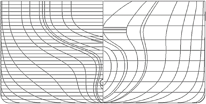Figure 3. Side view and body planes of the KVLCC2 ship model

As mentioned in the mathematical model section (2.1), the solver uses overset structured mesh for simulation. This allows application of high resolution near the hull surface and relatively lower resolution in the outer domain. The rectangular coarse outer mesh is used for capturing the free surface deformation and the O-H structured fine inner mesh is used for capturing the boundary layer near the hull surface. The inner domain is placed at a distance of 1.8L from the inlet or inflow boundary of the outer domain. The outflow or rear boundary of the outer domain stands at 2L distance from the end point of the inner domain. The inner domain maintains equal distance from the side boundaries of the outer domain. The inner, outer and combined mesh arrangement is shown in Figure 4. To avoid numerical exception, the back stern plate of the hull was slightly modified for the full hull simulations. However, the effect of this modification is minimum in the simulations, as explained by Islam [21] in his thesis.

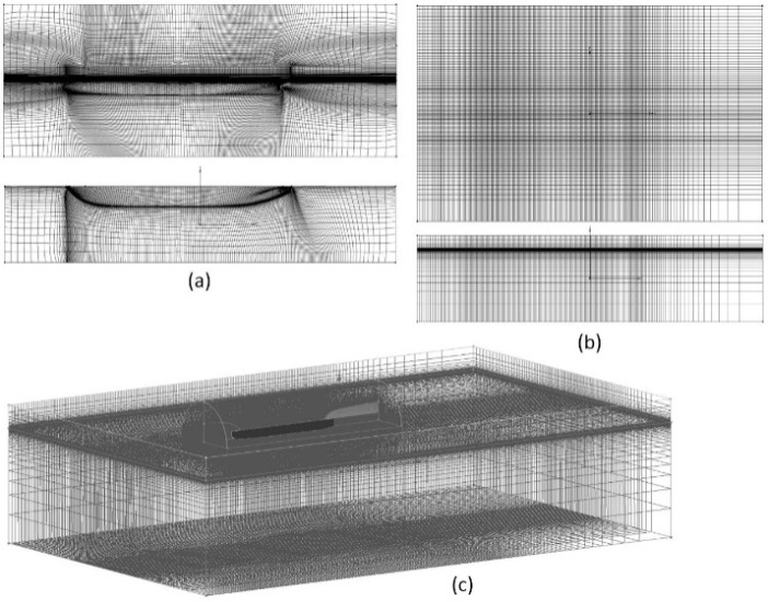Figure 4. Mesh arrangement used for simulation, (a) inner mesh domain (front and bottom view), (b) outer mesh domain (top and front view) and (c) combined mesh domains (isometric view)

In the case of mesh distribution in outer domain, gradually increasing spacing (roughly 150 times of near hull surface spacing) was used in both rear and side direction of the outer domain to dissipate the incoming waves in both head and oblique directions. The waves were generated from the starboard side, thus gradual spacing was applied at the port side, as illustrated in Figure 4(b). As the outer mesh distribution in port side and starboard side were different, a mirror image of the port side couldn’t be used. Thus, full outer domain (both starboard and port side) was provided. However, in the case of the inner domain, only port side mesh was provided as input and starboard side was generated using symmetry.

The simulations were limited to short wave cases because of the complexity involved in oblique wave simulations. With the increase in heave and pitch motion in oblique waves, attaining pressure convergence became very difficult. Furthermore, properly dampening the oblique wave using just numerical dissipation is quite challenging as well. To attain reliable results, relatively high mesh resolution was used, which further complicates things for oblique wave simulations, despite the used of overset mesh.

2.2.1. Computational Resource

The simple structured solver with zero-equation turbulence model and structured mesh around the bare hull was both light and fast in running simulation cases. However, the OpenMP memory sharing model used in the solver limited its capacity in distributing mesh information in multiple RAM modules. Thus, simulations were performed in a single node of Intel(R) Xeon(R) CPU with 8 cores, with 2.27 GHz of clock speed and 8 GB of physical memory. Despite the code’s lightness, oblique wave simulations were difficult to perform and required small time steps for convergence, which escalated the total time for simulation. The standard time step used was non-dimensional time and for simulating each non-dimensional time, the required physical time was about 90 hours per case. All the simulations were run up to 8 non-dimensional times for attaining stable results.

3. Results and Discussion

3.1. Added Resistance Prediction in Head Waves

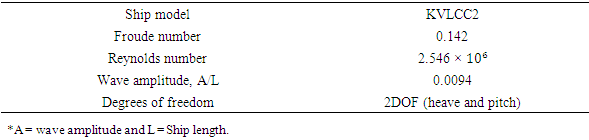
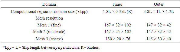
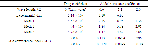
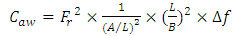
Added resistance is mainly the additional resistance a ship faces while forwarding through the waves. This additional resistance is encountered because of loss of energy in the radiated waves caused by the ship motion and the diffraction of incident waves on the ship hull. The energy distribution among these two components is dependent on the ratio of incident wave length to ship length (λ/L). For wave lengths up to half of the ship length, the main contributor to resistance is the reflection of incident waves at ship hull. In case of wave length being around ship length, ship’s heave and pitch motion mainly account for the principal resistance.

For added resistance calculation, sufficient mesh resolution is required at ship bow and stern part to properly capture the radiated waves, and near the water line at starboard and port side to capture the incident waves. Resolution and dimensions of the outer mesh are also important to capture the free surface deformation with reasonable accuracy.

In this research, three different mesh resolutions were used to investigate the mesh dependency of the solver. For discretization based uncertainly analysis, the procedure advised by Celik et al. [28] was used. For validation study, experimental fluid dynamics (EFD) data was taken from INSEAN, reported in the paper by Hosseini et al. [5]. Verification and validation study for the solver can also be found in the theses of Ock [29] and Islam [21]. Table 2 and Table 3 show the simulation conditions and the mesh resolution used for mesh dependency analysis and Table 4 show the results of simulations.

Table 2. Simulation conditions for the non-dimensional KVLCC2 model

Table 3. Simulation mesh configuration

Table 4. Simulation results and grid convergence for head wave cases

For conversion of simulation results to that of comparable state with EFD data, following conversion equations were used. Added resistance coefficient,

(15)

Where, Fr is the Froude number, B is ship's width and Δf is the difference between non-dimensional wave force and calm water drag force.

Heave Response Amplitude Operator (RAO),

(16)

Here, z is the heave amplitude, L is ship length and is incoming wave amplitude.

Pitch Response Amplitude Operator (RAO),

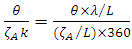(17)

Here, θ is pitch amplitude, L is ship length, is incoming wave amplitude and λ is the wave length.

The results show monotonous convergence for all cases. However, the grid convergence index were found to be relatively high for mesh 1 and 2, this might have been because of the low difference in mesh resolution between the two. Although the highest mesh resolution produces more agreeable results to the experimental data, the relative low different in mesh resolution but high difference in results between mesh 1 and 2 creates a higher level of uncertainty.

After grid dependency and uncertainty analysis, the moderate mesh resolution was used to perform simulations for short wave length cases. This was done to reduce simulation time and also to ensure convergence for complicated scenarios like oblique wave simulations. Test cases were kept limited to short wave cases, as in case of large ships like KVLCC2, it is very unlikely that such ships would voyage through a sea with λ/L greater than 0.8 [6]. For comparison, EFD data was taken from MOERI, reported in the paper by Kim et al. [6]. The mesh resolution and simulation conditions are stated in Table 5 and the results are shown in Figure 5 and Figure 6. In the figures, the red squares and blue triangles represent experimental data from MOERI and Osaka University, respectively. The green circles represent CFD data produced using WAVIS, an in-house RaNS code of MOERI. The gray circles and rectangles represent CFD data predicted using SHIP_Motion. The black line shown is the actual sea spectrum which corresponds to representative sea condition for EEDI weather. The same results were reported in a conference by Islam and Akimoto [30], however, it didn’t show the verification study. It can be seen from results that the CFD predictions show good agreement with both experimental and other simulation results.

Table 5. Simulation conditions and mesh resolution for the non-dimensional KVLCC2 model

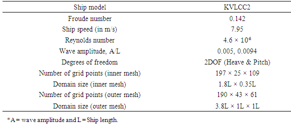
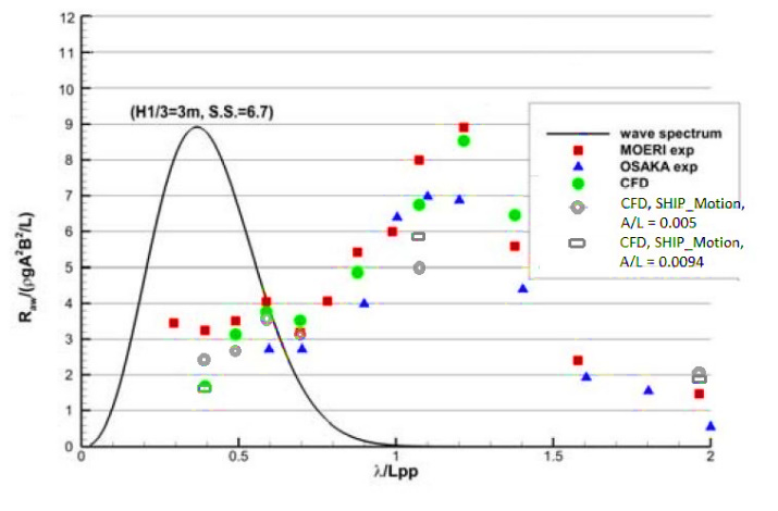Figure 5. Added resistance coefficient in head waves, CFD and EFD results (2DOF) [23]

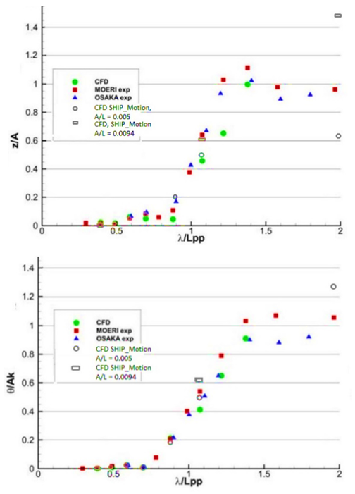Figure 6. Heave and Pitch RAO (respectively) for head wave simulation (2DOF) [23]

Nevertheless, in case of simulations in oblique waves, 2DOF may not be sufficient. In oblique waves, roll and sway motions become significant and they affect the resistance encountered by the ship in motion. Thus, considering higher degrees of freedom becomes essential. So, to check the dependency of results based on degrees of freedom, full hull simulations were performed with different degrees of freedom. The mesh resolution (twice of half hull resolution) and the simulation conditions were kept same as shown in Table 5, except the degrees of freedom. Simulations were performed for 2 (heave and pitch), 3 (heave, pitch, and roll), 5 (sway restricted) and 6 degrees of freedom of motion. The simulations were performed with the bare hull, without any appendages. Although in head waves, heave, pitch and surge motions are of primary importance, roll motion was prioritized here considering the oblique waves. Figure 7 shows the added resistance coefficient prediction in head waves for different degrees of freedom, and Figure 8 shows their heave and pitch RAOs. The experimental data was taken from MOERI [6]. As for time history of surge motion, it is not shown in this paper because of the absence of comparison data in given simulation conditions. These results on simulation dependency on degrees of freedom of motion were elaborately discussed by Islam and Akimoto [31] in a book chapter.

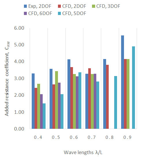Figure 7. Added resistance coefficient in head waves for different degrees of freedom of motion

The final simulations for oblique waves were performed only with 5 DOF. As tanker ships come with inherent low direction stability, if simulation is performed with all 6 DOF, without any rudder action, the ship loses its initial heading due to high yaw motion, as can be seen from Figure 9 (As the wave generation starts at 2 non-dimensional times, the simulation takes additional time, roughly 2 non-dimensional times, to reach stable motion). Thus, after λ/L= 0.7, simulation in 6DOF wasn’t continued.

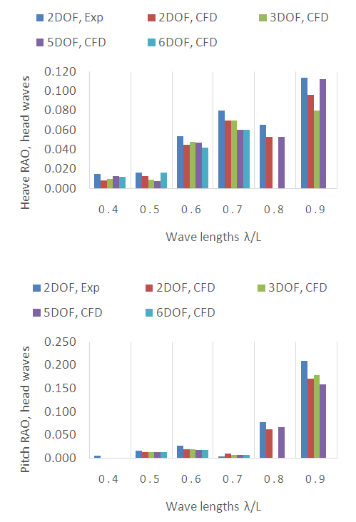Figure 8. Heave and Pitch RAO in head waves for different degrees of freedom, respectively

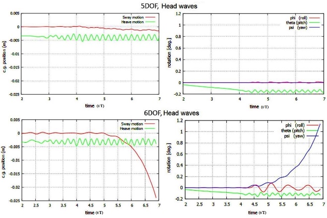Figure 9. Linear and rotational response of the KVLCC2 with 5DOF (above) and 6DOF (below) in head waves at λ/L = 0.7 and A/L = 0.005

The results show that the relative average difference among added resistance coefficient prediction for different DOFs is minor. For short wave length cases, the difference is very small; for λ/L=0.8, a higher deviation is observed, but the difference again minimizes at λ/L=0.9. Heave and pitch RAOs also show little variation with increased degrees of freedom. This is because, in case of resistance prediction, ship hull shape, and heave and pitch motions play most significant role. Roll motion is more important for checking habitability and yaw motion for predicting required rudder force. Thus, roll, sway, surge, and yaw adds minor changes to drag resistance and significant variations are not observed.

As for the deviation observed with experimental data, this was mainly because of the low mesh resolution in X-direction of the outer mesh. This was a compromise that had to be done in order to ensure convergence in oblique wave simulation cases. In oblique wave simulations, the incoming flow angle is changed, which makes convergence difficult to attend. The solution was, either to enlarge the mesh size or to decrease the time steps, to ensure the validity of CFL condition.

3.2. Added Resistance Prediction in Oblique Waves

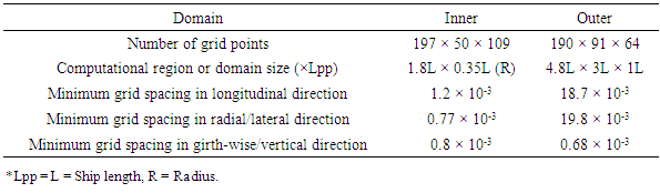
For added resistance prediction in waves, simulations were performed for three different wave directions, head waves and two bow wave directions. Simulation conditions remained the same as shown in Table 5, except that, the oblique wave simulations were performed with 5 DOF (yaw restricted). Mesh resolution used for running oblique wave simulations are shown in Table 6. The mesh resolutions are shown for full domains, for both inner and outer domains. The table also shows the minimum spacing applied near the wall boundary layer area. The spacing was gradually increased in longitudinal, radial and vertical direction, as the distance increased from the ship hull/wall surface.

Table 6. Simulation mesh configuration

In oblique waves, ship’s encountered wave length is different than the applied one. For this reason, a left ward (towards shorter wave lengths) shift is observed in curves of added resistance coefficient and pitch RAO vs wave length. The simplified encounter wave length concept used here can be explained using simple geometry. In Figure 10, β represents the oblique wave angle and λ_E, the effective wave length due to the oblique course. Thus, in head wave direction, if the observed wave length is λ; in case of oblique heading with angle β, the resultant wave length will be,

(18)

In this paper, head wave condition is represented by β = 180°; β = 150° and β = 120° represent a change of heading angle in the port direction by 30° and 60°.

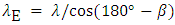
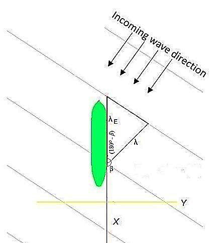Figure 10. Schematic diagram of oblique wave encounter by the ship

In head wave condition, the ship rides the wave with heave and pitch motion. Whereas, in case of the oblique waves, the waves are encountered mostly by one side of the hull. Thus, ship response changes. In this case, roll, sway, and yaw motion become significant. For this paper, oblique wave simulations were performed to observe the linear and rotational response of the ship in such conditions.

The added resistance coefficient predicted using simulation results for head and oblique waves are shown in Figure 11. As can be seen from the results, a leftward shift is observed in resistance coefficient prediction. A similar phenomenon has also been observed by Duan and Li [16] while performing potential flow based simulation on series 60 tanker ship.

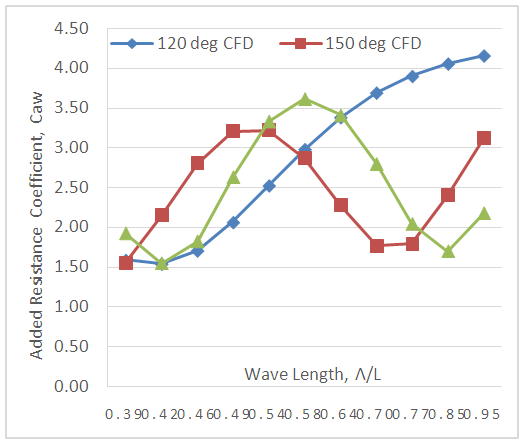
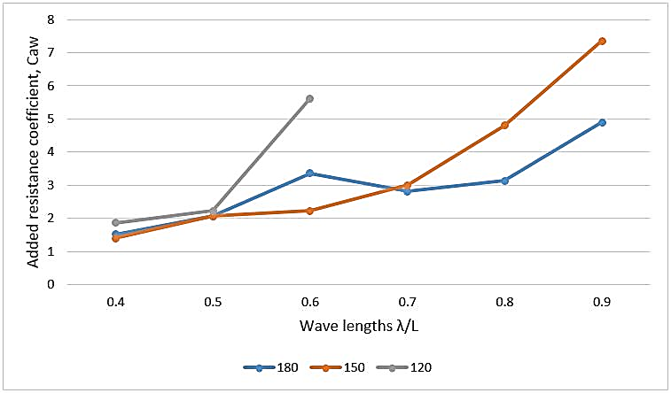Figure 11. Added resistance coefficient prediction for the KVLCC2 in head and oblique waves using SHIP_Motion

Results for heave RAO is shown in Figure 12 and for pitch RAO in Figure 13.

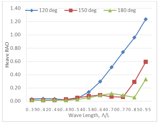
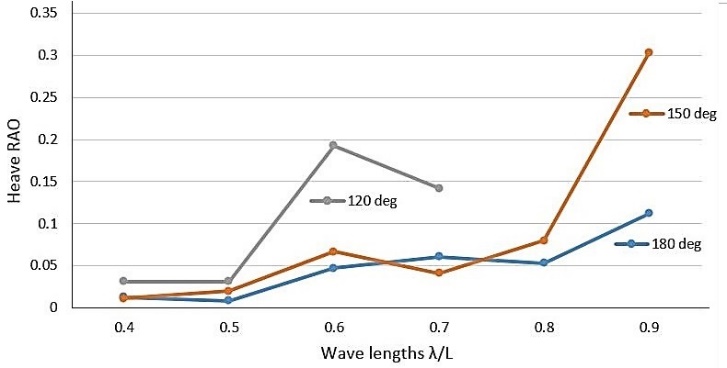Figure 12. Heave RAO prediction for the KVLCC2 in head and oblique waves using SHIP_Motion

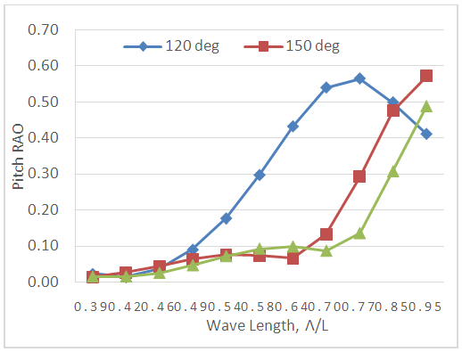
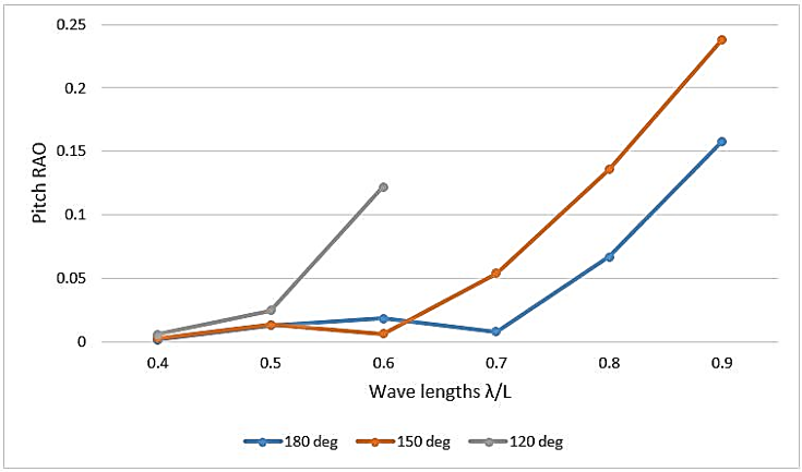Figure 13. Pitch RAO prediction for the KVLCC2 in head and oblique waves using SHIP_Motion

The leftward shift of results for oblique waves can partly be explained by the encountered wave lengths by the ship. In oblique waves, the encountered wave length is longer than the actual sea wave length, hence the leftward shift. The results may further be explained by the one-sided encounter of the wave by the hull, which results into high rolling, sway and yaw motion.

The linear and rotational motion response for simulation with 5DOF in the head and oblique waves for λ/L=0.6, A/L=0.005, are shown in Figure 14. As can be seen from the figure, in cases of oblique waves, the rotational motion increases significantly in oblique waves, as comparing to head wave simulation. The absence of linear sinusoidal motion in case of roll motion may be attributed to the short length waves, which continuously impact on the hull surface before one full roll motion is complete. Thus, humps are created on roll profile every time a wave hits the hull surface.

Figure 14. Linear and rotational motion response for the KVLCC2 in head and oblique wave simulation, with 5DOF, at λ/L=0.6 and A/L=0.005

To further confirm the findings, a commercial potential flow (PF) based solver named HydroStar [32, 33] was used. The solver is owned by Bureau Veritas and uses 3D panel method to solve 3D diffraction/radiation flow problems. However, the accuracy of the solver in predicting resistance is quite limited, thus, the results are shown here only as a comparison for trends. Figure 15 shows the trend for predicted added resistance coefficient in the head and oblique waves using HydroStar. Although the prediction for head wave case shows significant deviation from EFD (Figure 5), it captures the trend somewhat well. The same can be said for heave and pitch RAO prediction, as shown in Figure 16 and Figure 17. PF codes, in general, are efficient and reliable in predicting ship motion in head waves. However, in the case of oblique waves, non-linear behaviors are dominant, which limits the accuracy of potential codes. Here, direct comparison between RaNS and PF results are not shown since, PF simulations were performed in frequency domain, and wave lengths for the two cases do not match.

Figure 15. Added resistance coefficient prediction for the KVLCC2 in head and oblique waves using HydroStar

Figure 16. Heave RAO prediction for the KVLCC2 in head and oblique waves using HydroStar

Figure 17. Pitch RAO prediction for the KVLCC2 in head and oblique waves using HydroStar

3.3. Comparison of Flow Field in Head and Oblique Waves

In order to better understand the results, a comparison of ship motion response and flow field data is shown in this section. The comparisons are shown for encounter waves. That is, the comparisons are made for a particular wave length in head wave and for the same encounter wave length in oblique waves. This is done to show the hull’s response in head and oblique waves for same encountered wave length.

3.3.1. Comparison for Heading Angle of 150°

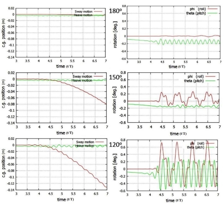
In case of heading angle of 150°, for an applied wave length of 0.6L, the encounter wave length is 0.7L (approx.). First, to check the difference in motion response of the ship in case of head waves and oblique waves, a relative comparison of motions is provided in Figure 18. The figure shows that, in case of head waves, the roll and sway motion is very limited. Whereas, in case of oblique waves, comparatively higher roll and sway motion can be observed. For oblique waves, pitch motion is also slightly different. The higher roll and sway motion is because of the encounter of incoming waves by one side of the hull.

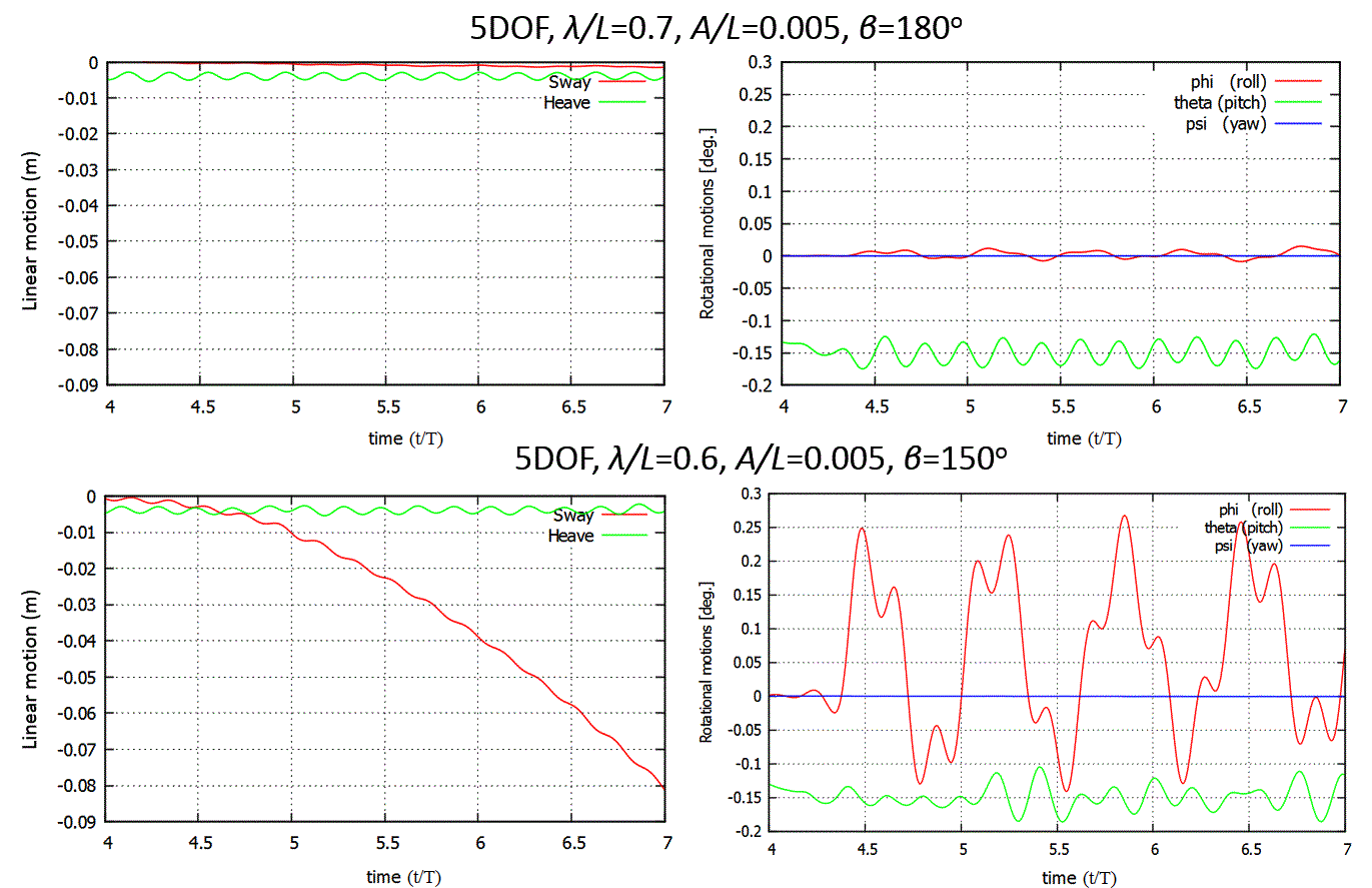Figure 18. Linear and rotational motion response of the KVLCC2 in simulation with applied wave length of 0.7L and 0.6L for head (β=180°) and oblique (β=150°) waves, respectively

Next, free surface deformation was observed by checking the free surface elevation for head (β=180°) and oblique (β=150°) waves. As can be observed from Figure 19, the free surface elevation in case of oblique waves is comparatively less than head waves. This can be explained by the one-sided wave encounter and reduced pitch motion of the ship. This indicates, less energy is dissipated on the free surface, thus, a lower resistance is encountered in the case of propagation through oblique waves.

It may be observed in Figure 19 that, there is a discontinuity in wave elevation in the intersection region between the inner and out domain. One of the reasons behind it is the difference in mesh resolution between the inner and outer domain at intersection region. While interpolating flow variables from inner to outer or outer to the inner domain, due to the difference in number of nodal points, the discrepancy is observed. Furthermore, the contours of domains overlap with each other there. With shorter time steps and maintaining similar resolution for the inner and outer domain, this discontinuity should reduce significantly. However, to reduce computational time, this was compromised for present simulations.

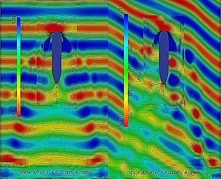Figure 19. Free surface elevation during propagation of the KVLCC2 through the head (β=180°) and oblique (β=150°) waves

Finally, pressure distribution on the hull surface for head (β=180°) and oblique (β=150°) waves was analyzed for checking the hull’s reaction in the head and oblique waves. Figure 20 shows the pressure distribution on ship hull surface (starboard and port side) while encountering the incoming waves. Naturally, in head wave condition, pressure distribution remains the same at starboard and port side. Still, both sides are shown for easy comparison with the oblique wave cases.

Next, in Figure 21, pressure distribution is shown in the starboard and port side of the hull in oblique wave condition. As can be observed from the figures, in oblique waves, pressure encountered by the starboard side is slightly higher as compared to head wave case. On the other hand, pressure on the port side of the ship is low. As a result, overall, the resistance encountered in oblique wave cases were found to be less, as compared to head wave cases.

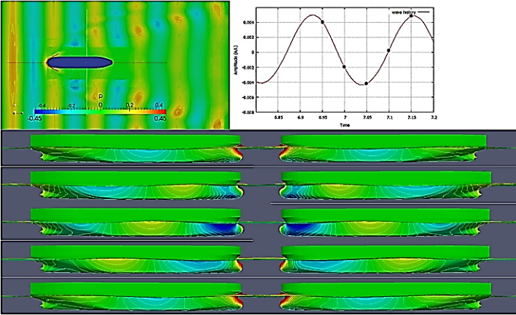Figure 20. Pressure distribution on hull surface of the KVLCC2 with 5DOF, at head waves (β=180°), λ/L = 0.7 and A/L = 0.005; starboard side (left) and port side (right)

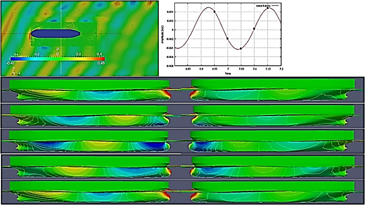Figure 21. Pressure distribution on hull surface of the KVLCC2 with 5DOF, for oblique waves at β = 150°, λ/L = 0.6 and A/L = 0.005; starboard side (left) and port side (right)

3.3.2. Comparison for Heading Angle of 120°

In case of heading angle of 120°, for an applied wave length of 0.4L, the encounter wave length is 0.8L. Similar to the previous case, first, to check the difference in motion response of the ship in case of head waves and oblique waves, a relative comparison of motions is provided in Figure 22 for wave amplitude 0.005L and 5DOF. The figure shows that, in case of head waves, the roll and sway motion is limited. Whereas, in case of oblique waves, comparatively higher roll and sway motion can be observed. As for lower pitch motion, in case of head waves, the ship shows wave riding motion. Whereas, in case of oblique waves, wave riding motion disappears as wave amplitudes are different at starboard and port side of the ship.

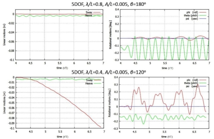Figure 22. Linear and rotational motion response of the KVLCC2 for applied wave length of 0.8L and 0.4L for head (β=180°) and oblique (β=150°) waves, respectively

Next, free surface deformation is observed (Figure 23) by checking the free surface elevation for head (β=180°) and oblique (β=120°) waves. As in the previous case, the free surface elevation in case of oblique waves was comparatively less than for head waves. Lower pitch motion also reduced energy loss. As a result, less energy dissipated on the free surface, thus, lower resistance was encountered in case of propagation through oblique waves.

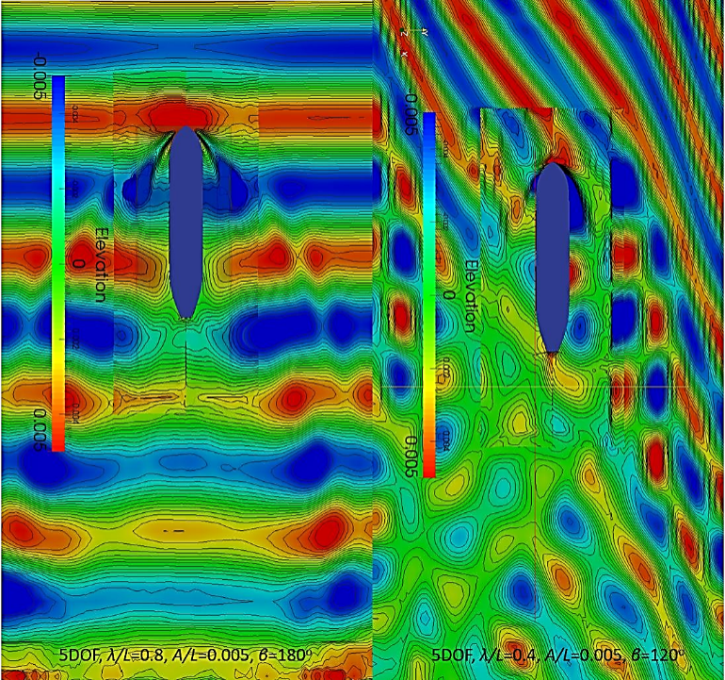Figure 23. Free surface elevation during propagation of the KVLCC2 through head (180°) and oblique (120°) waves

Finally, pressure distribution on the hull surface for head (β=180°) and oblique (β=120°) waves was analyzed for checking the hull’s reaction in the head and oblique waves. Figure 24 shows the pressure distribution on ship hull surface while encountering the incoming waves. Then, in Figure 25, pressure distribution is shown in the starboard and port side of the hull in oblique (β=120°) wave condition. As can be observed from the figure, in oblique waves, pressure encountered by the starboard side was slightly higher as compared to head wave case. On the other hand, pressure on the port side of the ship was comparatively very low. As a result, overall, the resistance encountered in oblique wave cases were found to be less as compared to head wave cases.

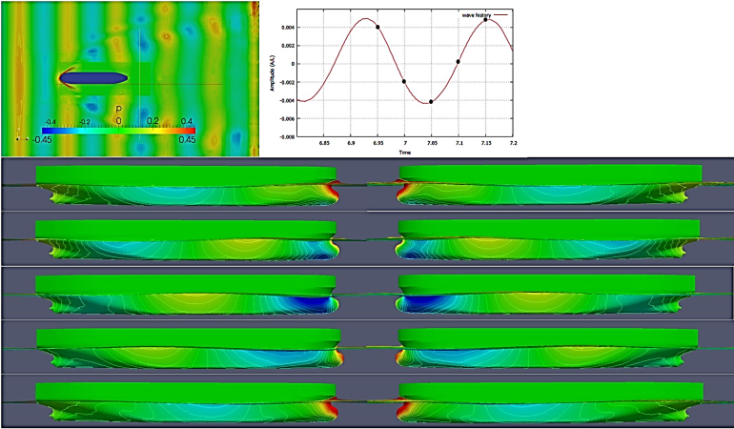Figure 24. Pressure distribution on hull surface of the KVLCC2 with 5DOF, at head waves (180°), λ/L = 0.8 and A/L = 0.005

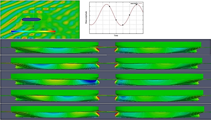Figure 25. Pressure distribution on hull surface of the KVLCC2 with 5DOF, for oblique waves at β= 120°, λ/L = 0.4 and A/L = 0.005; starboard side (left) and port side (right)

4. Conclusions

Simulations with 5DOF were performed for oblique wave cases for a tanker ship using RaNS solver and the results were compared with head wave simulation results based on encounter wave lengths. The results show that ship resistance and motion curve in oblique waves take a left ward shift (towards shorter wave lengths) with reduced amplitude comparing to head wave curves.

The added resistance encountered by the ship during its motion through the waves is mainly because of loss of energy in the radiated waves caused by the ship motion and the diffraction of incident waves on the ship hull. In case of ship motion in oblique waves, encounter waves are longer than actual length. Thus, even at short wave lengths, heave and pitch motions become important. The primary effect of oblique course is elongated encounter wave lengths and hence, the shift of resistance coefficient curve to shorter wave length direction. Besides leftward shift of resistance curve, a decrease in resistance coefficient is also observed. The reasons may be explained by the visualization figures. In case of oblique waves, the wave is encountered mostly by one side of the ship. As a result, it shows higher rolling motion but lower heave and pitch motion. The free surface deformation is also less in case of oblique waves. Thus, added resistance encountered by the ship is also less in oblique waves comparing the same encounter wave length in head waves.

The paper presented a case study to better understand how ship’s motion behavior and encountered resistance changes while facing oblique waves. Ship motion history and simulation flow field data were used to analyze the changes in ship resistance, and a PF code was used to reproduce simulation results to strengthen the claims. However, direct validation with experimental data is missing, and the number of cases presented in oblique waves were also limited. Thus, further work is need to improve our understanding on the topic.