1. Introduction

Humpback whales (Megaptera novaeangliae) are remarkable swimmers in oceans. These animals belong to rorquals (Balaenopteridae) under a broader group of cetacean mammalian marine animals. These giant swimmers possess a knobby head, a dorsal fin placed on two-third of the animal back surface, a powerful fluke and a streamlined body along with a long length about 12-18 m and a medium weight range among rorquals from 30 to 40 tons, compared to other heavy weight species like blue whales with about 140 tons [1, 2]. Humpback whales also exhibit a high level of swimming manoeuvrability in the ocean partially linked with their powerful flukes [1] and also superior hydrodynamic performance of their flippers with an approximate length of 0.3 of the body length and with special tubercled topology shown in Fig.1 [3, 4]. As one can observe in the figure, humpback whales have evolved tubercles on the leading edge and the trailing edge of their flippers representing a special pattern involving peaks and troughs with varying amplitude and wavelength [4].

Turbulent and transitional flows over tubercled wings have been extensively studied in the literature. As a short summary, wings with wavy leading edge planform depict superior lift coefficient performance in the after-stall region compared to the clean planforms [3, 5 and 6]. Streamwise vortex generation is a crucial factor to explain flow characteristics over a humpback whale flipper. In this case, wavy leading edge generates two counter-rotating vortices with different vorticity signs at different sides of the trough of each individual protuberance and secondary- spanwise flows are generated in the leading edge region. It is postulated that higher amount of momentum induced by streamwise vortices originating from protuberances results in a softer/ flatter post-stall behaviour for wings with leading edge undulations [5, 6].

Caused by the ecological constrains of life in oceans, humpback whales have also developed some unique individual and social behavioural features, like breaching behaviour (Fig.1), generation of the most complex sound among the swimming animals in general and in their group foraging process [7, 8] and utilization of a smart bubble net hunting technique [9], to name a few [2].

Figure 1. Humpback whale flipper; Top: breaching behaviour [15], Bottom: flow pathlines obtained from turbulent flow simulations over a humpback whale flipper model constructed based on a real flipper planform at angle of attack (AoA) [3]

In the latter bubble net fishing method, humpback whales exhibit a very clever and corporative social behaviour by generation of bubble columns (with an approximate diameter of 4-7 m) and bubble clouds (1-1.5 m) to maintain naturally concentrations of prey, as clarified by Hain et al. [9].

In general, humpback whales feed on crustaceans, krill and also various fishes. In lunge feeding process, which happens in few seconds, they expand their throats like an accordion multiple times of its resting statue (Fig. 2) and then cruise into the prey concentration zone with an open mouth to engulf huge amount of prey-laden water [10-13]; this is done with the aid of opening of their ventral pleats supported by their strong ventral cavity multi-layer muscles [14]. Afterwards, ocean water bulk filtering phase is performed at the beginning of the digestive process. All rorquals have ventral grooves on the bottom-side of their body.

From hydro-dynamical point of view, presence of these grooves modifies the external shape of the bottom-side humpback whales, even in the non-lunge stage formed by longitudinal folds of skin, compared to the smooth body surface, which can affect swimming performance of the aquatic animal (Fig. 2).

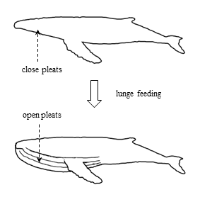Figure 2. Humpback whale lunge feeding process

Fig. 2 shows a schematic picture of the lunge feeding process of humpback whales; there exists two modes, including ‘close’ and ‘open’ pleats. As one can see in the figure, pleated throat (or mouth cavity) of the animal are extended to multiple times of the initial size; in this way, humpback whale is able to engulf enormous amount of prey-laden sea water, but at the expense of high energy cost induced by high amount of drag force [11]. As shown by Goldbogen et al. [11] in a similar case of fin whales, engulfed mass is approximately proportional to , where is the body length of the whale. For instance, for a whale with total length of 14 and 16 m, amount of engulfed mass of prey-laden ocean water would be approximately equals to 15 and 24 tons, respectively. It is also worth mentioning that by increasing the body length, engulfed mass capacity of the aquatic animal increases; furthermore, oxygen carrying capacity of these air-breathing marine animals improves by increasing the size of these breath-hold divers, providing them more time at foraging depth [13].

There exist many interesting lessons considering humpback whale swimming hydrodynamics; however in this paper, hydrodynamics of external turbulent flow passing over the humpback whale ventral pleats is studied. In this regard, flow fields around a simplified model of the animal body are numerically simulated at different angles of attack (AoA, hereafter) and a prescribed sideslip angle. In the following, details are presented.

2. Humpback Whale Body Model

Ellipsoid can be considered as a good approximation to represent the streamlined body shape of many cetaceans. As shown in the top view of a humpback body sample in Fig. 3, a 3:1 ellipsoid can be adopted to model main features of the humpback whale body, as hired in this paper.

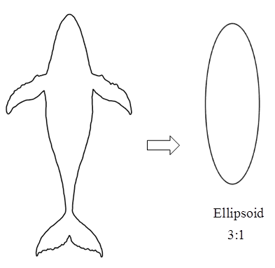Figure 3. Humpback whale body approximation

Geometrically, ventral grooves can be characterized as semi-parallel lines on the elliptic Riemannian geometry of the bell surface with a positive curvature. Therefore, semi-parallel groove lines (curves) create a diverging- converging pattern with a varying angle with respect to the longitudinal body axis as shown in Fig. 4-top [16]. It is also worth to mention that ventral pleat pattern is a unique sign of any individual humpback whale specie, similar to fingerprints for human being.

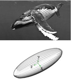Figure 4. Humpback whale body; Top: non-lunge swimming (modified from the original picture [16]), Bottom: simplified body model as an ellipsoid with ventral pleats on the half of the body surface

The bottom picture in Fig. 4 shows isometric view of the constructed simplified humpback whale body utilized for the upcoming grooved body flow simulations. The model consists of a base 3:1 ellipsoid with minor and major diameters equal to 0.1 and 0.3 m, respectively. The model also involves ventral pleats each with a depth of and a width equals to , where is the local radius of a circle formed by intersection of the vertical planes perpendicular to z-axis and the ellipsoid, while is equal to . To construct the geometry a total number of 20 intersection curves and 2 guide curves forming the external shape of the ellipsoid in the plane, defined by y=0, are generated by high resolution and imported into the SolidWorks CAD environment. Then, the resulting half- grooved ellipsoid model resembling humpback whale body is majorly constructed by utilizing a lofting process, i.e. stitching the guide curves by surfaces, as shown in Fig. 4.

3. Numerical Methodology

To study flow field details over the grooved and non-grooved ellipsoids, numerical simulations are conducted at different AoAs and a given sideslip angle. In all simulations, the body model is kept at a fixed position in space, i.e. in y-z and x-z planes and effects of AoA, , (Fig. 5-a) and sideslip angle, , (Fig. 5-b) are included via setting freestream blowing angles, i.e. and (Fig. 5).

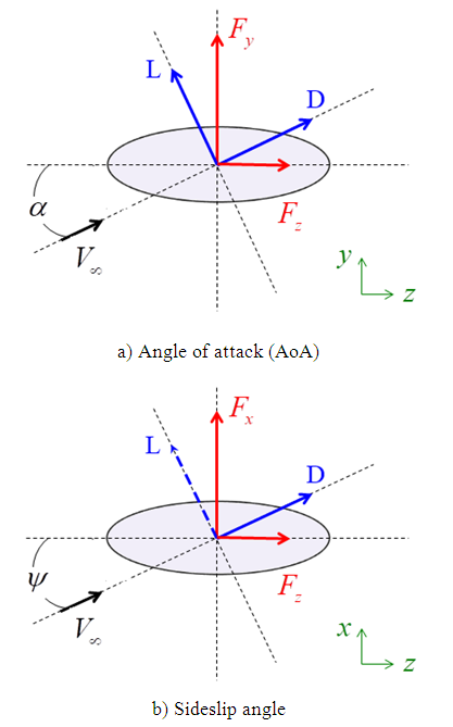Figure 5. Coordinate system utilized for the ellipsoid simulations

As one can see in Fig.5, there is a rotational transformation to translate forces in the y and z directions (Fig. 5- a) in y-z plane and also in the x and z directions (Fig. 5- b) in x-z plane (calculated directly in the simulations) to lift and drag forces. This is simply done by matrix manipulations. Inflow velocity at the inlet plane is also imposed by three components of the velocity, defined via a prescribed Reynolds number . For inflow setting with AoA in y-z plane, freestream uniformly flows in x-direction by imposing null lateral velocity at the inlet plane, as below:

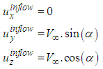(1)

while for inflow setting with sideslip angle in x-z plane, freestream uniformly flows in y-direction by imposing null vertical velocity at the inlet plane, as below:

(2)

Freestream velocity is also set by a predefined . Humpback whales with a body length about 12-18 m, experience turbulent flows on their body, with high easily reaching to orders of magnitude equal to 10⁷-10⁸. To have an idea, maximum swimming speed of the humpback whales while singing is about 4 m/s [17] and in general with maximum about 7 m/s and minimum of about 0.55-2.0 m/s in the feeding phase; in addition, ocean current speed is fastest near the ocean surface with about 2.5 m/s and gulf currents speed is about 1.8 m/s [18]. As an example, for a humpback whale with a typical length of 15 m, swimming with speed of about 1 m/s, is equal to , defined based on the body length. In this paper, all upcoming ellipsoid simulations are performed at this Reynolds number, i.e. .

3.1. Computational Domain and Mesh Generation

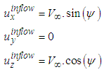
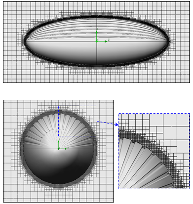
To investigate hydrodynamic effects of the humpback whale ventral grooves, two series of simulations are performed on the constructed models in this study: first, a 3:1 ellipsoid without grooves, namely ‘clean’ ellipsoid hereafter, and second a 3:1 ellipsoid with pleats on half-surface of the body namely ‘grooved’ ellipsoid hereafter, resembling ventral pleated body of humpback whales (Fig. 4- bottom). As mentioned in the previous section, both geometries have been numerically constructed in SolidWorks CAD Environment [19]. Computational grids for these external flow simulations were also constructed using SolidWorks meshing tools with Cartesian-base grid coupled with an adaptive mesh- clustering to capture complex geometrical features like ventral pleats and also boundary layer zone, with minimum 10 nodes close to the wall in the boundary layer [20].

Fig. 6 depicts grid generation around the clean ellipsoid along with the computational domain. For the grooved ellipsoid, computational domain is exactly the same as Fig. 6-top, except in the near body zone, where mesh is modified by ventral grooves, as shown in Fig. 7. The latter figure shows front and side views of the generated grid for the grooved ellipsoid in the middle sections of the ellipsoid which exhibits clustering to the wall. As shown in both Fig. 6 and Fig. 7, near wall zone is completely well-captured to the wall due to the computational demand of the utilized turbulence treatment in the present study (soon explained in the next subsection). After performing grid convergence test, two well-converged grids with about 1.5 and 2 million elements have been utilized for the clean and grooved ellipsoid simulations, respectively. It is worth mentioning that running simulations resolving to the wall for multiple operating points adopted in this study is computationally costly; therefore, there always exists a trade-off between size of the computational domain, mesh resolution and the desired achievable accuracy.

Figure 6. Clean ellipsoid grid and computational domain

Figure 7. Grooved ellipsoid cross-sectional grids at the middle planes: side view (top) and front view (bottom)

As one can also see in Fig. 6 (top), computational domain is considered large enough about two times of the ellipsoid major diameter in the streamwise (z) and lateral directions (x and y directions) to minimize the boundary effects. As also stated before, computational domains for the both ellipsoids have the same size and configuration as Fig.6 (top).

3.2. Flow Solver, Turbulence Treatment and Settings

In unsteady Reynold averaged Navier-Stokes (URANS) approach, governing equations of fluid motions including Navier-Stokes, continuity and also turbulence model equations are numerically solved in the case of turbulent flow simulations. In this paper, the governing equations of non- cavitating and cavitating turbulent flows over the humpback whale body model are solved using SolidWorks Flow Simulation (SFS) solver [19, 20] with Lam-Bremhorst low- Reynolds number version of model (LB LRN , hereafter), resolving to the wall [21]. In general, fluid flow governing equations of the problem can be expressed as below [20, 22]:

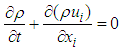(3)

(4)

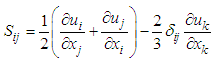
where the last term, , is the source term and total stress tensor , including Reynolds stress tensor, is defined as the following:

(5)

(6)

In the above equations, and denote turbulent eddy viscosity, turbulent kinetic energy and Kronecker delta, respectively. The above set of equations suffers from a so-called ‘closure problem’; therefore, the extra variable, i.e. turbulent eddy viscosity, should be estimated in a way. In LB LRN like the original model, this is done by solving two extra transport equations for turbulent kinetic energy and turbulent eddy dissipation coupled with the aforementioned governing equations, as below [20, 21 and 22]:

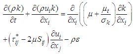(7)

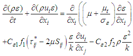(8)

where some ad-hoc parameters in the LB LRN similar to the original are empirically set, as below:

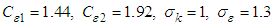Having on hand both and values at each computational node, turbulent eddy viscosity is calculated as:

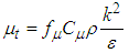(9)

where and LB damping function , also and parameters (Eq. 8) in the LB LRN version of the model are defined as below:

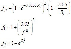(10)

where the intermediate parameters in the above equations are defined as below:

(11)

where is defined as the shortest distance to any solid surface. Finally time and length scales of the representative turbulent eddy at each computational node can be computed using the following relations [23]:

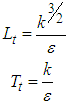(12)

As observed in the above equations, the modified model utilized here is different with the original turbulence model; in LB LRN approach, damping functions, and also and functions are introduced and calculated as functions of the minimum distance to the wall. In addition, it is worth mentioning that SFS needs at least 10 nodes in the direction normal to the wall-surface in the boundary layers to efficiently approximate these high gradient zones with LB LRN method [19, 20].

In non-cavitating cases, finite-volume SFS solver numerically solves governing equations of the fluid flow motions by an operator-splitting technique and uses a SIMPLE-like approach to treat pressure-velocity decoupling issue [19, 20]. Furthermore, the solver solves asymmetric linear system of the discretised equations coming from the momentum/ turbulence with a preconditioned conjugate gradient method along with an incomplete LU factorization preconditioning; while symmetric pressure-correction system of equations is solved by the aid of a multigrid technique [20].

In cavitating cases, SFS uses another all-speed solver developed based on a hybrid density- and pressure-based splitting technique proposed by Alexandrikova et al. [22]. The underlying method adopts a separate density-based approach for compressible flow zones, while uses a pressure-based treatment for incompressible zones without cavitation simultaneously in a single computational domain [22]. Furthermore, the solver uses the same LB LRN turbulence model as explained before along with a barotropic state equation as , derived with thermodynamic equilibrium assumption [22]. With the aid of the smart underlying splitting technique, SFS is capable to handle a broad range of time scale, density and speed of sound variations, arising in a single domain in cavitating flow conditions.

As mentioned earlier, for numerical simulations three components of the inflow velocity (Eq. 1 or 2) are set at the inflow section. Other boundaries are treated as ‘outflows’. For simulation convergence, predefined goals as and forces (or equivalently lift and drag forces) are monitored on top of the velocity and pressure variables to achieve a converged state; in SFS solver, convergence criteria is automatically set by the solver based on dynamic calculation of dispersion of the goal functions, which guarantees the lowest convergence residual level [19]. In the next section, simulation results are presented in details.

4. Results and Discussion

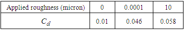
In this section, turbulent flows over the humpback whale pleated body model, i.e. the grooved ellipsoid, are simulated at high Reynolds number, . There is no experimental data available in this case; therefore the effects of ventral pleats are studied by comparison to results of the turbulent flow simulations over the clean 3:1 ellipsoid model. To perform flow simulations over the clean and grooved ellipsoids, first of all effects of applied surface roughness is considered to adjust the parameter for the upcoming simulations. Table 1 depicts drag coefficient values obtained from turbulent flow simulations on the clean ellipsoid at null AoA, , for different applied averaged roughness values. As it is clear in the table, a roughness equals to 10 microns results in a drag coefficient close to the ellipsoid experimental value, i.e. [24, 25]. For both clean and grooved ellipsoids in all upcoming simulations, an averaged roughness value of 10 microns is applied.

Table 1. Drag coefficient obtained from numerical simulations of the clean ellipsoid at different roughness values

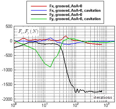
4.1. Streamwise Humpback Whale Swimming

In this subsection, streamwise swimming of humpback whale is modelled by non-cavitating turbulent flow simulations of the grooved body along with the clean body for comparison purposes at . Due to the symmetry exists in the case of clean ellipsoid at , one can expect to have null lift force in this case. Fig. 8 shows and force oscillations around zero as convergence history of the goal function for the clean ellipsoid. Fig. 9 similarly shows lateral forces variations for the grooved ellipsoid compared to the clean one. As one can see in the latter figure, in contrast to the previous case, the grooved ellipsoid generates noticeable amount of force and contributes to lift generation (here like buoyancy force in the negative-y direction) of the animal. The difference observed between the clean and grooved ellipsoids are expected a-priori, due to symmetry breakdown existing in the grooved case in y-direction.

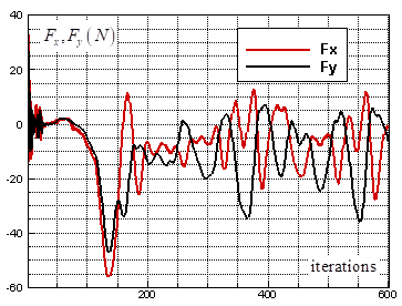Figure 8. Lateral force goal function history for the clean ellipsoid at

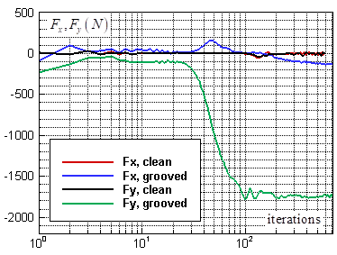Figure 9. Lateral force goal function history for the grooved and clean ellipsoids at

As also shown in Fig. 9, is also generated for the grooved ellipsoid, due to the dissymmetry imposed in x-direction to partially mimic the natural dissymmetry existing in the real ventral groove pattern of a humpback whale (Fig. 7). Fig. 10 shows variations of the axial force for both clean and grooved ellipsoids.

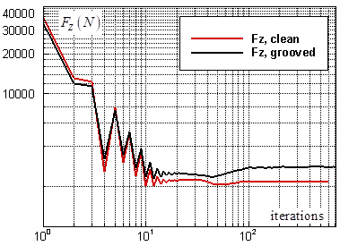Figure 10. Axial force goal function history for the grooved and clean ellipsoids at

As one can see in Fig. 10, the grooved ellipsoid exhibits higher level of the ultimate axial force (here drag force) compared to the clean ellipsoid; this is directly translated to the higher level of drag coefficient of the grooved ellipsoid compared to the clean one 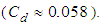In Fig. 11, front view of axial velocity field along with pathlines in the middle section, defined by z=0, is shown.

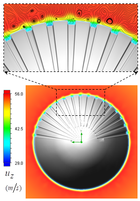Figure 11. Axial velocity field around the body at in the middle plane at z=0: pathlines close to the body (top), front view (bottom)

It should be kept in mind that for better visibility in the figures, the grooved surface is typically shown upward, although in horizontal swimming of a humpback whale as an example, the surface with the ventral pleats is in the bottom of the animal, i.e. downward; in this sense, negative contributes to buoyancy force and should be interpreted as a lift force, i.e. opposite to the animal weight force. By comparing top and bottom surfaces of the body in Fig. 11, one can obviously observe that ventral grooves modify the velocity field pattern compared to the clean surface in the bottom; in fact, strip of low velocity form on the bottom surface of the animal body. Fig. 12 also shows axial velocity field in the longitudinal middle plane defined as x=0.

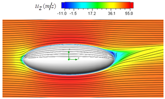Figure 12. Axial velocity field around the body at in the middle plane defined as x=0

As one can see in Fig. 12, symmetry between top and bottom regions breaks due to presence of the ventral pleats on the top surface. As expected, a stagnation point at the ellipsoid nose is present and also an asymmetric recirculation zone forms at the aft-body zone of the grooved ellipsoid. To capture hidden structures in the flow field like vortical structures/shear layers, -criterion is utilized here [26]. The -criterion method links the minimum extrema of pressure occurring in vortex core regions or shear layers in the case of shear contamination to the eigenvalues of the Hessian of pressure, i.e. 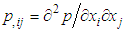; in the method vortex cores with/without shear contamination can be identified by . In fact, the threshold level utilized for capturing the structures is case-dependent and is typically selected by try and error. Fig. 13 depicts hidden structures generated on the humpback whale body simplified model obtained via -criterion with threshold as .

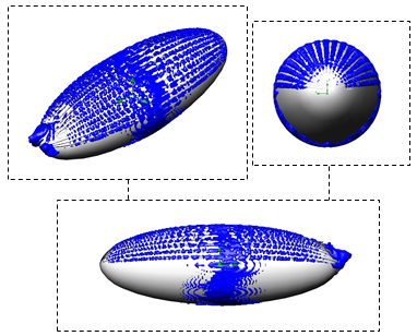Figure 13. Vortical structures/shear layers developed on the humpback whale body model captured by -criterion at : isometric view (top-left), front view (top-right) and side view (bottom)

As one can see in Fig. 13, vortical shear structures form on the pleated surface of the humpback body model. These shear structures generate low-speed strips on the humpback whale body, which in turn generates relatively higher local pressure zones close to the body (Fig. 14); in this manner, negative is generated that contributes to buoyancy force in humpback whale swimming at the expense of more energy consumption due to higher level of drag force (table 2).

Table 2. Summary of numerical performance coefficients for the grooved and clean ellipsoids

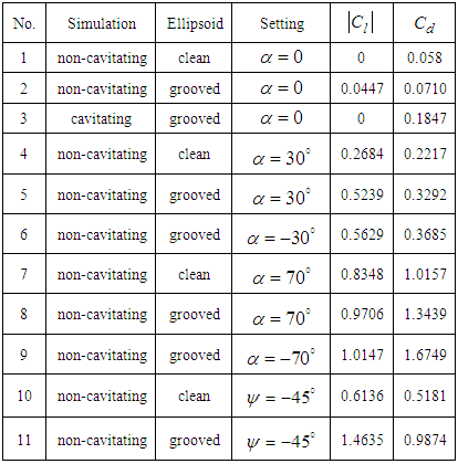
Figure 14. Pressure field on the clean (right) and grooved (left) surfaces of the humpback whale body at

To see fluid particle motions under hidden structures formed in the flow field especially in cases involving high AoA and sideslip angle in the next subsections, tracer particle studies are performed. Fig. 15 shows a snapshot of the tracer motions coloured by axial velocity of the particles in the streamwise swimming.

Figure 15. Isometric view of tracer particle dynamics over the humpback whale body in the streamwise swimming

In this regard, tracer particles, here ethane spherical particles with 0.0001 m diameter are continually released from the humpback whale body surface and convected downstream by the background flow field. In contrast to ideal tracers, real tracers applied here have mass and do not have the same velocity as local flow; therefore, equations of motion for those particles are solved under a given velocity field. For the calculations here, ideal reflection has been applied for fluid particle-solid interactions, e.g. in the recirculation zones. As one can see in Fig. 15, tracer particles smoothly move over the body surface at this null AoA and partially enter into the recirculation zone at aft-body zone which depicts more complicated movements. As shown shortly, dynamical motions of tracer particles at higher AoA and sideslip angle exhibit a chaotic over the body, especially in the recirculation and vortical structure zones.

4.2. Effects of AoA

Despite having a giant body and mass, humpback whales unexpectedly exhibit high level of manoeuvrability in rolling, banking and turning; as mentioned this is majorly linked to their unique tubercled flipper [3, 4]. These swimming animals experience a broad range of AoA and sideslip in their manoeuvres in the oceans; to complete the picture and to study hydrodynamic effects of the pleated body in the flow field a set of different AoA and a sideslip angle are considered for simulations in the present and next subsections, respectively, as 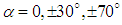and . Table 2 summarizes numerical performance coefficients, i.e. lift and drag coefficients covering all numerical simulations performed in this paper. As one can see in the table, for all AoA, lift coefficient obtained from the grooved body is higher than the corresponding coefficient of the clean ellipsoid, while the grooved body results in a higher level of drag coefficient, majorly due to the formation of low-speed shear strips in the grooves. It is also observed in the table that by increasing AoA, lift and drag coefficients increase as expected. The symmetry also breaks for positive and negative AoA, due to presence of the ventral pleats on the half-surface of the body and as a result of geometrical symmetry breakdown in y- direction with respect to the plane, defined by .

In Fig. 16 and Fig. 17, convergence history of the axial and lateral forces for different AoA values, 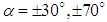, are shown. As one can see in the figures, behaviour of the grooved and clean ellipsoids is different at the same AoA, as expected. In addition, in the case of grooved ellipsoid resembling humpback whale body, there is no symmetry between cases; the same dissymmetry is also observed between cases; as stated before, this difference comes from presence of the ventral grooves on the half of the wetted surface. As one can see in the both figures, for the clean ellipsoid, and are also generated at both positive and negative AoA, although absolute values of the forces are obviously less than the corresponding values in the case of the grooved ellipsoid. It is trivial that positive and negative AoA in the case of clean ellipsoid have the same behaviour due to its geometrical symmetry (not shown).

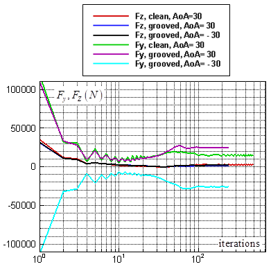Figure 16. Axial and lateral force goal function monitoring for the grooved and clean ellipsoids at

Figure 17. Axial and lateral force goal function monitoring for the grooved and clean ellipsoids at

As it is also visible by comparing Fig. 16 and Fig. 17, absolute values of the converged forces i.e. and increase by increasing AoA. In table 2, all ultimate converged force data are translated to the lift and drag coefficients. Fig. 18 shows topology of the flows at different AoA.

As one can see in Fig. 18, at higher AoA more complicated flow pattern is illustrated by flow pathlines bundling around the grooved body, due to formation of vortical structures in the wake of the body. As also shown in the figure, there is no symmetry between cases; in the negative AoA, pathlines are getting more bundled than in the positive AoA and forms a heavy wake due to presence of ventral pleats on the top surface. The effect is less pronounced in the cases, although still exists.

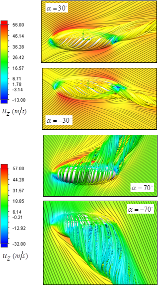Figure 18. 3D pathlines over the grooved body along with the axial velocity field in the middle plane defined as x=0, at different AoA

Fig. 19 shows front view of averaged flow field at ; as shown in the figure, a region of high velocity forms on top of the body. Two counter-rotating vortices are also generated on the grooved surface.

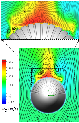Figure 19. Axial velocity field around the body at in the middle plane at z=0: pathlines close to the body (top), front view (bottom)

To further investigate the hidden governing flow structures in the flow fields at different positive and negative AoA, -criterion is applied. Threshold levels as and are applied for and , respectively. As one can observe in Fig. 20, different structures form on the grooved surface at different AoA. At , two attached tail-like vortical structures with positive and negative angle with respect to the longitudinal axis of the body, i.e. z-direction are generated at positive and negative AoA, respectively. For both cases, structures form on the grooved surface; although at , structures are extended to the clean surface as well. By increasing AoA to , few scattered and shorter tails are generated at the aft-body. In addition, an attached structure forms originating from the ellipsoid nose. At , tail structures are efficiently omitted and only covering structures on the grooved surface are generated along with two relatively short spikes at the ellipsoid nose, as shown in Fig. 20.

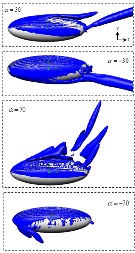Figure 20. Vortical structures/shear layers developed on the humpback whale body model (side view) captured by -criterion at different AoA

Presence of the grooves on the ellipsoid surface also modify size of the representative turbulent eddies on the body. This concept can be investigated by looking at the turbulent length scale (, defined in Eq. 12) on the body surface; smaller turbulent structures are typically generated on the grooved surface on the top compared to the clean surface of the body on the bottom, as shown in Fig. 21 for as an example.

Fig. 21 also shows shear stress variation on the humpback whale body model at ; as it is obvious in the figure, high shear stress strips form on the grooved surface on the top, while the clean surface possesses very low values of the shear stress due to formation of large separation zone on the bottom at this AoA.

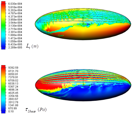Figure 21. Turbulent length scale (top) and shear stress (bottom) fields on the humpback whale body surface at (side view)

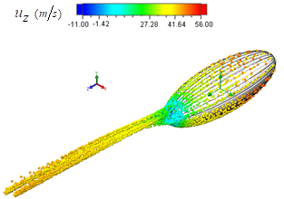
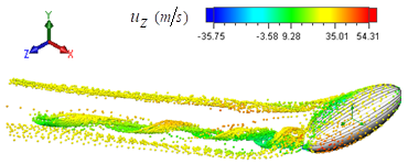
To have a better feeling about the fluid particle motions in the flow field under the governing hidden structures, tracer particle studies are performed at different AoAs similar to the aforementioned particle study performed at . Like before, spherical ethane particles with 0.0001 m diameter are released from the humpback whale body surface and convected downstream by the background flow field. Ideal reflection has also been applied for fluid particle-solid interactions, e.g. in the recirculation zones. As an example, Fig. 22 depicts a snapshot of tracer particle motions at . As one can see in the figure and also in a movie generated by the present particle study, tracer particles majorly follow vortical structures arising on the grooved surfaces and pass downstream.

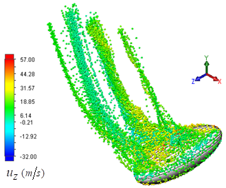Figure 22. Particle dynamics study over the humpback whale body at

4.3. Effects of Sideslip Angle

Humpback whales experience high angles of sideslip in their manoeuvers in the oceans. In this subsection, turbulent flow over the body is simulated at high sideslip angle, i.e. , as shown in Fig. 23.

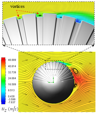Figure 23. Axial velocity field around the body at in the middle plane at z=0: pathlines close to the body (top), front view (bottom)

Fig. 23 shows formation of counter-rotating vortices on the right side of the body and also vortical structures in the groove cavities. 3D Pathlines around the body are also shown in Fig. 24 in this case; as one can see in the figure, pathlines are deflected due to applying the sideslip angle.

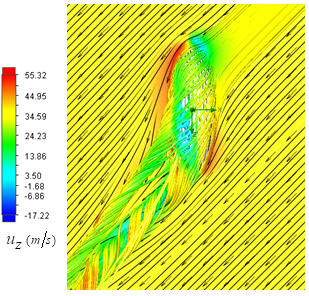Figure 24. 3D pathlines over the grooved body along with the axial velocity field in the middle plane defined as y=0, at

As it is obvious in table.2, the grooved ellipsoid exhibit’s a superior lift coefficient performance compared to the clean ellipsoid in flow conditions with sideslip angles, but at the expense of a more drag-based energy consumption; quantitatively, lift coefficient improves from 0.6136 for the clean ellipsoid to 1.3645 in the case of the grooved body and drag coefficient also increases from 0.5181 to 0.9874 for these cases, respectively. It is worth mentioning that for the clean ellipsoid, lift force is generated in x-z plane for inflows with sideslip angle; but for the grooved ellipsoid, due to symmetry breakdown in y-direction, lift is not kept in x-z plane and follows the direction of resultant combination vector of and component projections of and . Fig. 25 shows convergence history of forces in the case of flow over the grooved ellipsoid at .

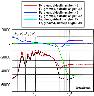Figure 25. Axial and lateral force goal function monitoring for the grooved and clean ellipsoids at

As shown in the latter figure, force convergence is achieved earlier in the case of grooved ellipsoid compared to the clean ellipsoid. As mentioned about Fig.24, pathlines are deflected due to presence of sideslip angle; in addition, hidden flow structures are deflected in this case. Fig. 26 shows tracer particle dynamics under the deflected hidden structures; in this case, three major vortical paths are generated on the body and extended downstream.

Figure 26. Isometric view of tracer particle dynamics over the humpback whale body at sideslip angle as

At sideslip angle , turbulent length scales are also modified on the clean and grooved surfaces as shown in Fig. 27. As one can see in the figure, at x⁺ larger turbulent eddies are generated compared to the turbulent structures at x^- on the clean surface. In general, finer turbulent eddies are generated on the grooved surface compared to the clean one, similar to the typical cases investigated in this paper at other AoAs; a strip of large vortices is also generated at x^- in the aft-body zone on the grooved surface as shown in Fig. 27.

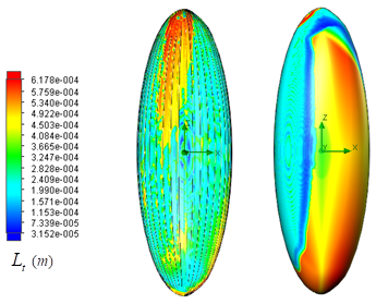Figure 27. Turbulent length scale field on the clean (right) and grooved (left) surfaces of the humpback whale body at

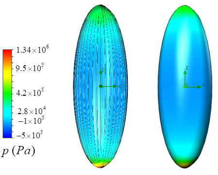
4.4. Swimming in Cavitating Conditions

As mentioned earlier, some groups of humpback whales learned to use a social foraging technique, called bubble net feeding, for prey haunting [7, 8, 9, and 27]. In the process, they move in a shrinking helical/circular path, with a dimeter of about 3 to 30 meters, towards the surface blowing air rings/cloud at different instants from beneath of a prey school via two blowholes of these breath-hold swimming animals to make the prey more concentrated. They basically control pattern of the bubble column cylinder via bubble generation characteristics; in general, there is a continuous trade-off between net depth and bubble generation characteristics due to different rise rates of small and large bubbles, as showed in details by F. A. Sharpe [27]. After fish schooling provided by the resulting bubble net and forcing the prey to concentrate moving upward, at the next step humpback whales swim upward in a drag-based feeding fashion, i.e. mouth open, to engulf the prey colony. In this process, humpback whales basically swim in an air and water mixture, not in a pure-water condition. On the other hand, there always exist some sorts of dissolved gas in the ocean/sea water [28].

In general, flow simulation in multiphase flow conditions is a challenging task due to existence of a broad range of Mach number and time scales of the phenomena involved. In fact, sonic speed dramatically drops in air-bubble and water mixture; as an example, speed of sound in liquid sea water is about 1500 m/s and in water-vapour is about 450 m/s depending on the temperature; for liquid-vapour mixture, speed of sound drops to about 3.2 m/s at volume fraction of 0.5 [29]. In the case of air-water mixture with air volume fraction of 0.4, sonic speed drops to about 20 m/s [30]. By local decreasing of sonic speed in different regions of a single computational domain, solver encounters to local Mach number increase and even presence of shock waves in the solution domain. As explained in section 3.2, to handle cavitating flows, an all-speed solver developed based on a hybrid density- and pressure-based splitting technique along with LB LRN turbulence treatment are hired in the solver.

In this section, to have an idea about hydrodynamic effects of ventral pleats on the humpback whale body in a bubble net environment, a cavitating flow simulation is performed at with having inflow dissolved gas mass fraction of 0.001. Fig. 28 shows density variation around the humpback whale body model along with tracer particle dynamics coloured by axial velocity quantity.

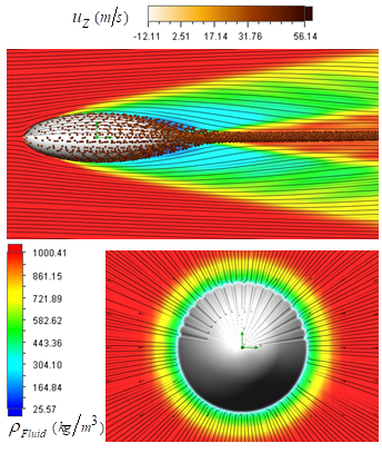Figure 28. Cavitating flow field around the body: fluid density superimposed with tracer particle dynamics, side view (top), front view (bottom)

As one can see in the figure, radical density variations from liquid water density, i.e. 1000 kg/m³, to vapour water, i.e. 25.27 kg/m³, encounter through the formation of a shock- wave system around the body at this high Reynolds number. Particle study with ethane particles with 0.0001 m diameter in Fig. 28 reveals formation of a more concentrated wake behind the body compared to the non-cavitating conditions (Fig. 15). Fig. 29 shows variations of the lateral forces on the grooved body; As shown in the figure by comparing the black and green curves, in the case of cavitating flow condition, e.g. in the bubble net fishing environment, lift generation by the grooved body is suppressed.

Figure 29. Lateral force goal function monitoring for the grooved ellipsoid in the cavitating flow condition at

This issue can also be seen in table. 2, as lift coefficient favourably drops from 0.0447 to 0 in the cavitating flow condition. In fact, in bubble net hunting method humpback whales swim upward towards the concentred prey colony with the aid of their powerful irregular knobbly edge fluke; any generation of lateral forces in this situation can be viewed as a noise. Suppression of the lateral force generation in cavitating conditions facilitates directional control of the whales in the bubble net hunting technique. Fig. 30 shows flow structures captured by -criterion in the cavitating flow simulation at . As one can see in the figure, a similar but noisier structure pattern to the non-cavitating case (Fig. 13) is generated on the grooved ellipsoid in the cavitating condition. Here, density of the structures is higher in front-body region and less in the aft-body zone.

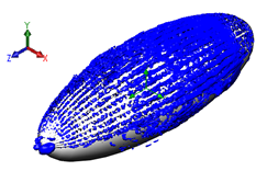Figure 30. Developed structures on the humpback whale body model identified by -criterion in cavitating flow simulation at

4.5. Predicted Separation Zones

To see the effects of ventral grooves on the separation zone fomation, separated flow regions, defined as , on the clean and grooved ellipsoids are shown in Fig. 31 and Fig. 32, respectively. As one can see in the both figures, by increasing AoA, larger separation zone form on the body.

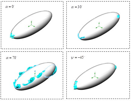Figure 31. Separation zones on the clean ellipsoid body at different AoA and a sideslip angle

As also seen in Fig. 32, symmetry between positive and negative AoA breaks in the case of the grooved ellipsoids, e.g. at , due to the geometrical dissymmetry in the y-direction generated by presence of the ventral grooves. By comparing Fig. 31 and Fig. 32 at , a long separated tail detached to the body is seen for the grooved ellipsoid, which is not present in the case of the clean ellipsoid; this reverse-flow zone is induced in the core filament of the strong vortical structure seen in Fig. 20 and also in the tracer particle dynamic study presented in Fig. 22. As one can also see in Fig. 32 at , a large separation zone is generated under the body on the clean surface due to presence of the ventral grooves on the top surface.

In the case of cavitating flow condition on the grooved ellipsoid at , separation zone depicts a very small reverse-flow region at the aft-body zone; the region is smaller compared to the non-cavitating case (Fig. 32). By comparing cases at , very close patterns are obtained for these positive and negative AoA; although small differences is still visible in Fig. 32. At , a relatively larger separation zone is generated at the aft-body zone; while small separations exist on the top at .

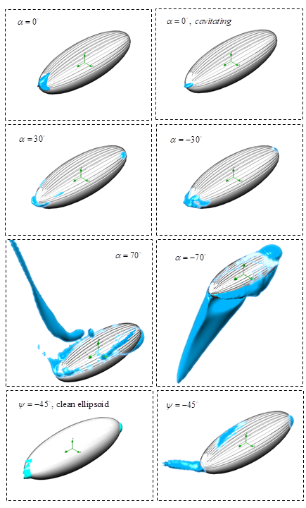Figure 32. Separation zones on the grooved ellipsoid body at different positive and negative AoA and a sideslip angle

In the case of flow with a sideslip angle equals to , a relatively similar pattern of separation lakes is obtained for the clean and grooved ellipsoids; although a deflected tail forms in the case of the grooved ellipsoid (Fig. 32), which is not present in another case (Fig. 1). Furthermore, a separation zone is generated on top of the body on the grooved ellipsoid (Fig.32), which does not exist on the clean ellipsoid body surface (Fig. 31).

It is also interesting to notice that due to a typical streamlined body developed by humpback whales under necessity of life in oceans, as modelled by a 3:1 grooved ellipsoid, large separation formation is only limited to high AoA.

5. Conclusions

In the present study, hydrodynamic effects of the ventral pleats covering bottom surface of the humpback whale body were studied for the first time. Although, the focus was put on the humpback whales in this paper, many other rorqual whale species also possess ventral pleats on the bottom surface of the body; therefore a similar conclusion can be made in those cases as well. Fig. 33 shows a schematic summary of the essential hydrodynamic effects of the ventral peats. As it is clear in the figure, ventral grooves on the right-hand side of the body are virtually removed to create an imaginary- smooth belly surface for comparison purposes only; offcourse in real species, ventral pleat net covers the entire humpback whale bottom surface.

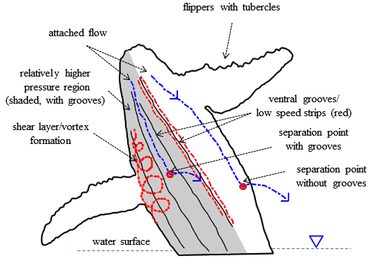Figure 33. Summary of hydrodynamic effects of humpback whale ventral pleats in the animal swimming

First of all, presence of the ventral pleats leads to the formation of relatively low-speed strips generating shear/ vortical structures in the grooves. These low-speed regions in turn generate relatively higher local pressure zones close to the body which contributes to buoyancy force generation by the body for non-cavitating flow conditions. This is also directly translated to higher lift coefficient for the grooved ellipsoid body model compared to the clean ellipsoid for all AoA examined in this study at the expense of a higher drag coefficient. In the non-lunge phase, these low- speed stripes also increase tendency of the flow separation. It was also seen that in the case of the grooved humpback whale body model, symmetry between positive and negative AoA breaks, e.g. for .

As shown in the paper, the grooved body exhibits a superior lift generation performance compared to the clean ellipsoid for flows with sideslip angle, e.g. ; at this sideslip angle, lift and drag coefficients increases about 138% and 90%, respectively, due to presence of the ventral grooves on the half of the body surface. Relative symmetry of the turbulent length scale in the lateral direction, i.e. x-direction, also breaks in the turbulent flow over the body with a sideslip angle.

It was also observed that turbulent length scale reduces on the grooved surface compared to the clean surface of the grooved ellipsoid for all AoA; in other words, smaller turbulent eddies are generated on the grooved surface. Particle studies performed at high AoA and at a predefined sideslip angle also showed complicated tracer particle motions in the separated zone and under vortical structures attached and detached to the body, induced due to the presence of ventral grooves on the body.

In the cavitating flow condition, resembling bubble net environment in this paper, swimming of humpback whales governed by their powerful fluke motion was considered at . Results showed that lift generation by the grooved surface is majorly suppressed under cavitating flow conditions; in other words, lift coefficient approaches zero and effects of grooves are effectively omitted in lift coefficient, although drag coefficient considerably increases in this situation; this provides a better directional control for the animal in the hunting final step by cancelling the lateral forces. As also shown, separation zone formation is modified by presence of ventral grooves on the humpback whale body.