-
Paper Information
- Paper Submission
-
Journal Information
- About This Journal
- Editorial Board
- Current Issue
- Archive
- Author Guidelines
- Contact Us
American Journal of Fluid Dynamics
p-ISSN: 2168-4707 e-ISSN: 2168-4715
2017; 7(1): 23-40
doi:10.5923/j.ajfd.20170701.03

MHD Flow of Cellulose Derivatives and Dilute Suspensions Rheology of Its Nanocrystals
 Abstract
 Reference
 Full-Text PDF
 Full-text HTML
S. E. E. Hamza
Physics Department, Faculty of Science, Benha University, Benha, Egypt
Correspondence to: S. E. E. Hamza, Physics Department, Faculty of Science, Benha University, Benha, Egypt.
| Email: |  |
Copyright © 2017 Scientific & Academic Publishing. All Rights Reserved.
This work is licensed under the Creative Commons Attribution International License (CC BY).
http://creativecommons.org/licenses/by/4.0/

The study of cellulose derivatives and magnetic field effects on their rheological properties (magnetorheological) is of evident practical importance because its ability to orient under the action of external fields. The orientation process is of great importance owing to the possibility of changes in structure and final products. The aim of this work was to study theoretically the effects of magnetic field on rheological behavior of some cellulose derivatives solutions. The studied samples are Ethyl cellulose (EC), Hydroxyethyl cellulose (HEC), Hydroxypropyl cellulose (HPC) and Carboxymethyl cellulose (CMC) dissolved in a suitable solvents. The influence of eight different solvents on solutions viscosity was investigated. Vshivkov and his group at the Department of Macromolecular Compounds at the Ural Federal University investigated experimentally the changes in magnetorheological properties of these solutions by using a Rheotest RN 4.1 rheometer. Their works covered the shear rates  and concentration range from to . In this paper, we reconsider Vshivkov et al. works through collecting their experimental data and carry out its theoretical analysis based on Giesekus model for viscoelastic polymers. This model gives more accurate results and takes into account the effects of viscoelastic shear thinning characteristics, decreasing viscosity with increasing shear rate. The regions of existence of isotropic and anisotropic phases and their concentration dependence were discussed. It is found that a magnetic field increases the viscosities of all solutions under consideration. The study was extended to report the viscosity data of dilute aqueous suspension of cellulose nanocrystals (CNC). It has been treated as a dilute fiber suspension whose concentrations ranging from 0.5 to 8 wt% and its rheology are analyzed using Giesekus model. The orientation of CNC nanoparticles are described in terms of the fiber's second– and fourth–order orientation tensors established by Advani and Tucker. Finally, for adequate prediction of viscoelastic shear thinning characteristics of CNC suspensions as a function of both shear rate and concentration, simple correlations were proposed in terms of an exponential function.
Keywords: MHD, Cellulose derivatives, Dilute Fiber suspension, Cellulose nanocrystals, Giesekus model
Cite this paper: S. E. E. Hamza, MHD Flow of Cellulose Derivatives and Dilute Suspensions Rheology of Its Nanocrystals, American Journal of Fluid Dynamics, Vol. 7 No. 1, 2017, pp. 23-40. doi: 10.5923/j.ajfd.20170701.03.
Article Outline
1. Introduction
- Cellulose is the most abundant polymer on Earth, which makes it the most common organic compound. It is the primary constituent of wood, paper and cotton. Cellulose is linear and rigid polymer consisting of a cyclic structure of anhydroglucose units. When these units are hooked together, the structure of cellulose becomes as shown in Fig. 1a. The chemical character and reactivity of cellulose is determined by the presence of three hydroxyl (OH) groups in the glucose units, one primary and two secondary groups. The hydroxyl groups play an important role in the solubility of cellulose. The relative stiffness and rigidity of the cellulose molecule is mainly due to the intramolecular hydrogen bonding. This property is reflected in its high viscosity in solution, a high tendency to crystallize, and its ability to form fibrillar strands. Cellulose chains have a strong tendency to aggregate and to form highly ordered structures and structural entities. The history of the supramolecular structure of cellulose, started as early as 1913 when Nishikawa and Ono discovered the structure of fibrous cellulose by the well–defined X–ray diffraction patterns [1]. This finding lead to the conclusion that individual cellulose molecules tend to arrange themselves in a highly organized manner leading to a crystalline state. Based on these findings, scientists developed the fringed fibrillar model of the structure, which is still accepted theory of the supramolecular structure. As shown in Fig. 1b, the latticework represents the highly ordered (crystalline) region whereas elongated lines represent the low ordered (amorphous) regions. The supramolecular model of cellulose is based on the organization of cellulose chains into a parallel arrangements of crystallites and crystallite strands, which are the basic elements of the CNC fiber [2]. The intermolecular hydrogen bonding are considered to be the major contributors to the structure of cellulose, and is regarded as the predominant factor responsible for uniform packing [3]. Today experimental evidence describes a two–phase model, which clearly divides the supramolecular structure into two regions: low ordered (amorphous) and highly ordered (crystalline) excluding the medium ordered regions completely [4].While unmodified cellulose is insoluble in water, modification of the cellulose chain by attachment of small substituents may result in water solubility properties. Published information suggests that, the secondary hydroxyl present in a side chain is available for reaction with the oxide and chaining out may take place. In 1956, Flory [5] predicted that polymers with stiff linear chains would form ordered phases in their respective melt and in concentrated solutions. In 1980, this behaviour was reported for cellulose derivatives, such as HPC in water, which at high concentrations can reflect visible light due to its nematic structure [6]. HPC was also the first cellulosic derivative reported to form spontaneous anisotropic solutions when dissolved in aqueous and organic solvents [7]. Since that discovery, other cellulose derivatives including: ethyl cellulose (EC), HEC, CMC, and cellulose itself have also been reported to form ordered solutions [8-14].When cellulose is etherified, the hydroxyls (OH) are replaced by the etherifying reagent. The final product is characterized by the degree of substitution (DS) which it is the average number of hydroxyls substituted per unhydroglucose unit. Therefore, EC is a derivative of cellulose in which some of the hydroxyl groups on the repeating glucose units are converted into ethyl ether groups. The properties of EC, as those of other cellulose derivatives, depend primarily up on the degree of substitution. It is practically insoluble in water but is soluble in varying proportions in certain organic solvents [15, 16]. While some solvents are excellent in dissolving EC polymer, they have limited or no application in the pharmaceutical industry because of their unacceptable effect on environment and health. EC find use in many applications, e.g. as water binders, film forming agents and in controlled release [17, 18]. They have been used in the fields of biotechnology, paints and foods [19-21]. Although interest in aqueous dispersions of ECs continues to interest, solvent–based EC extended release coating applications also continue to grow. The pure CMC is white or milk white fibrous powder or particles, odorless and tasteless. It is insoluble in organic solvents such as methanol, alcohol, diethyl ether, acetone, chloroform and benzene but soluble in water. Water solubility of CMC is affected by its DS and viscosity.
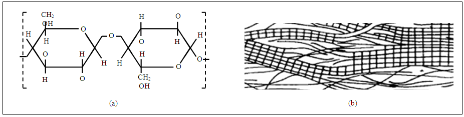 | Figure 1. (a) Structure of cellulose, (b) Fringed fibril model of the supramolecular structure of cellulose |
2. Problem Formulation
2.1. Governing Equations for Cellulose Derivatives
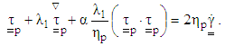
- In the present paper, circular Couette flow occurs in the gap between two rotating concentric cylinders rheometer is investigated. The inner cylinder of radius
 rotates with constant angular velocity
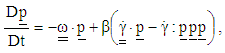
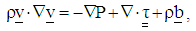
  . The apparatus has a height L which is much larger than the radius of either cylinder, see Fig. 2. In general, the momentum and continuity equations of steady MHD flow of incompressible viscoelastic fluid are given by:
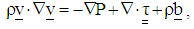 | (1) |
 | (2) |
 , and
, and are respectively the density, velocity, pressure, extra stress tensor and the body force per unit mass. Notice that, in the presence of an applied magnetic field, the term
 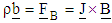 represents the Lorentz force due to magnetic field where
  is the current density and
  is the magnetic induction vector.
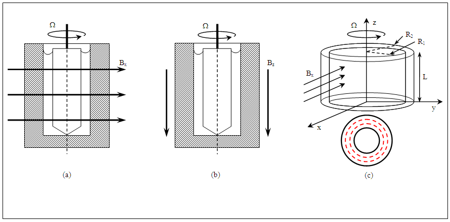 | Figure 2. Schematic representation of viscosity determination with magnetic lines of force directed (a, c) perpendicular and (b) parallel to the rotational axis of the rotor |
 for this model can be written as [44-46]:
 | (3) |
 | (4) |
 | (5) |
 is decomposed into a polymer contribution
  and a Newtonian solvent contribution
  . Also
 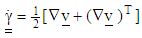 denotes the shear tensor and the superscript
  stands for the upper–convected derivative. The parameters
  and
and  are the solvent and polymer contributions to the zero–shear–rate viscosity,
  is relaxation time and α denotes Giesekus mobility factor
  . It is convenient to rewrite Eqs. (3) to (5) as a single constitutive equation by replacing
  in the last equation with
  . This leads to:
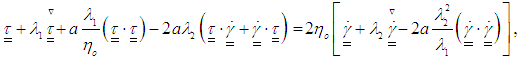 | (6) |
 is the zero shear rate viscosity,
  is the retardation time and “a” is the modified mobility parameter. These parameters are related through the relations:
 | (7) |
 is added .The inclusion of
  term in Eq. (6) gives material functions that are more realistic than any other model. For example, large decreases in the viscosity and normal stress coefficients with increasing shear rate are possible.In the present study, a cylindrical coordinate system
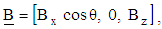
  is used. The magnetic field is applied either in x– or in z–direction as shown in Fig. 2 such that
  . From the physics of this problem, the flow is assumed to be axisymmetric
  . Therefore, the velocity field, magnetic field vector and the stress tensor can be written as:
 | (8a) |
 | (8b) |
 | (8c) |
 | (9) |
 and
and  are the strength of an imposed uniform magnetic field in r–and z–directions respectively. With these simplifications, the momentum equation reduces to:
 | (10) |
 | (11) |
 . The velocity at outer cylinder vanishes,
  , while at the surface of the inner cylinder is:
 | (12) |
 in Eq. (6) make it more difficult to obtain analytical solutions for the mathematical functions.
2.2. Viscosity and Elastic Characteristics
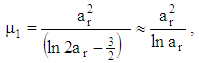
- Experimental analysis of shear rate dependent viscosity for cellulose derivatives solutions and dilute suspensions of CNC requires high accuracy measurements, because viscosities of these materials only slightly exceed those of the solvents. This is one of the reasons why viscometric studies are essentially absent for dilute polymer solutions. Something of the shear dependent viscosity of dilute polymer solutions can be gained from experiments [47]. An important problem in this field is the establishment of rheological characteristics that determine hydrodynamic behavior of polymeric solutions, and development of techniques for measuring these characteristics. Maxwell's and Jeffrey's models of viscoelastic fluids are very simple and unable for the behavior description of the dilute polymer solutions.Giesekus model is characterizes by four parameters
 ,
,  ,
,  and a, which can be treated as the model's parameters. Limiting cases of the Giesekus model include the Newtonian fluid
  , the upper–convected Maxwell fluid
  and the Oldroyd–B fluid
  . However, by adding a small retardation term
  , the magnitude of the shear stress is always increasing with increasing shear rate. In general we must require
  for realistic shear thinning and
  for shear thickening fluids and in general
  . Giesekus model yields the following material functions (apparent viscosity η, first and the second normal stresses
  and
and  ); [46]:
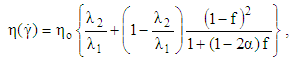 | (13) |
 | (14) |
 | (15) |
 | (16) |
 | (17) |
 and
and  are not taken into account here because of they can be measured only in un–symmetric regions such as eccentric cylinders or cone and plate rheometers. From this survey one can expect that sufficient realistic results will be observed for dilute solutions. It can thus be assumed that Giesekus model can be used in determination all rheological properties of cellulose derivatives and dilute CNC suspensions.
3. Governing Equations
3.1. CNC Suspension as a Fiber
- The rheological properties are the results of interaction among CNC fibers in the suspension flow. The volume fraction
 (total volume of CNC fiber in a unit volume of suspension) and aspect ratio
  (ratio of CNC fiber length to diameter) are two parameters influencing the rheological properties of suspensions. CNC Fiber interactions depend on its concentration,
  , and length. Hence, suspensions are classified according to its concentration as [48, 49]:
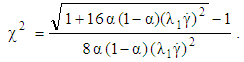
 | (18) |
3.2. CNC Fiber Orientation Description
- The properties of CNC fiber suspension are highly dependent on the orientation of the CNC fibers in its flow domain. The orientation of a single CNC fiber within a continuous medium matrix can be described in spherical coordinate system by the unit vector
 aligned along the axis of the CNC fiber as shown in Fig. 3, where
  is parallel to the major axis of CNC fiber with components:
 | (19) |
 .
.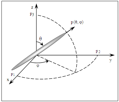 | Figure 3. Orientation of a single CNC fiber |
 whose value gives the probability of CNC fiber oriented between the angles
  and
and  and
and  and
and  as:
as: | (20) |
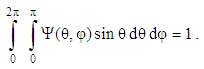 | (21) |
 is a complete description if the orientation of a single CNC fiber is unrelated to any other neighboring fibers. However, the calculations with the distribution function are too computationally cost when applied to industrially relevant flows. Therefore, the introducing of orientation tensors is a suitable way for describing the orientation state of CNC fibers. The orientation tensors are defined as [43, 52],
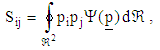 | (22) |
 is the unit sphere. The second–order tensor
  consists of nine components, however, due to symmetry
  the components is reduced to six. These tensor components can be written as:
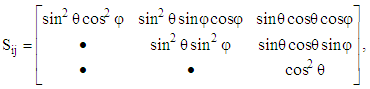 | (23) |
 have all information needed to describe the CNC fiber orientation. The normalization condition in Eqs (21) show the two fundamental symmetry properties of
  :
: | (24) |
 | (25) |
 | (26) |
 is simply:
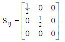 | (27) |
 is written as:
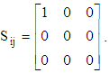 | (28) |
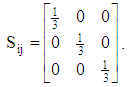
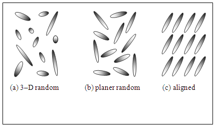 | Figure 4. Example of different CNC fiber orientation states |
 | (29) |
 as:
as: | (30) |
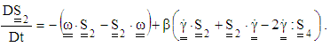
 . In Eqs. (29),
  is the material time derivative,
 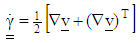 is the shear rate or deformation tensor and
  is the vorticity tensor. Instead of performing the integration and tedious calculation of the distribution function, an equivalent system of differential equations can be written that characterizes the orientation evaluation in terms of the tensors
  as:
as: 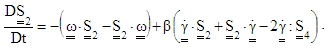 | (31) |
 in Eq. (31) contains
  . Thus, one needs a closure approximation to close the set of the evolution equations of the orientation tensors. A fourth–order closure may be expressed as:
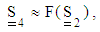 | (32) |
 . There are many methods proposed to address the closure problem. Most types of closure approximations is the linear one which originally introduced by Hand [53]:
 | (33) |
 is the unit tensor and
  refers to a space dimensions; i.e.,
  | (34) |
 | (35) |
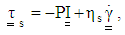
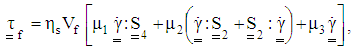
3.3. Constitutive Equation for CNC Fiber Suspensions
- Several constitutive models have been proposed to describe the stress tensor for a suspension of CNC fibers in a Newtonian fluid. In general, the total extra stress tensor for the suspension,
 , is taken to be the sum of the stress contributions from the Newtonian solvent fluid
  , and from the fiber,
  . Hence, the resulting constitutive equations for the suspension can be expressed as [54]:
 | (36) |
 | (37) |
 | (38) |

 are positive material parameters specified by the particle aspect ratio,
  . For a slender shape, particle thickness can be ignored producing
  and
and  equal to zero. Therefore, typical CNC fiber stress tensor for dilute CNC suspensions can be expressed as:
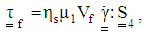 | (39) |
 | (40) |
3.4. Governing Equations for CNC Suspensions
- The total system of the CNC suspensions are governed by the following steady state equations:§ The equation of conservation of linear momentum; Cauchy's dynamical equation of motion,
 | (41) |
 | (42) |
 | (43) |
4. Test Materials
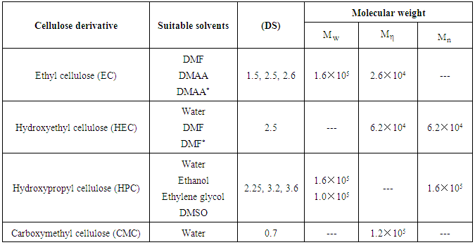
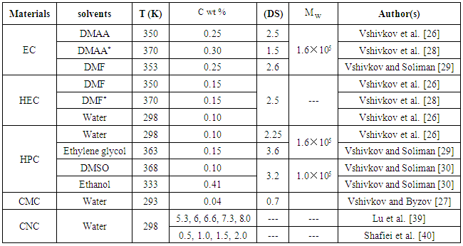
- From the end of the 2008s, systematic research onto magnetorheological of cellulose derivatives have been performed at the Department of Macromolecular Compounds at the Ural Federal University. The effects of shear rate, magnetic field and concentration on the rheological properties of cellulose derivatives were described by Vshivkov et al. [26-30]. The studied samples of cellulose derivatives are: EC, HEC, HPC and CMC. The used solvents were DMAA, DMAA* (DMAA with macromolecules), DMF, DMSO, ethylene glycol and ethanol.The corresponding author, molecular weight
 , DS and the used solvents for each cellulose derivatives are listed in Table 2. The solvent purity was studied through refractive index measurements [26]. The authors were prepared polymer solutions in sealed ampoules at certain temperature and concentration for several weeks.
|
 and dialyzed to remove the salts. Finally, the suspension was dispersed in an ultrasonic bath to achieve a 1-2 wt% concentration stable suspension. CNC particles were obtained in powder form by lyophilizing the suspension. The aqueous nanoparticles suspensions at different fiber concentrations (5.3, 6, 6.6, 7.3, 8 wt% [39] and 0.5, 1, 1.5, 2 wt% [40]) were then prepared and characterized in this study.
 5. Viscosity Measurements
- Vshivkov and his groups investigated experimentally the changes in magnetorheological properties of cellulose derivatives solutions by using a Rheotest RN 4.1 rheometer over shear rates
 . Their works covered the concentration range from 0.04 to
  . Figure 5 shows schematic representation of Rheotest RN 4.1 rheometer and its installation method in magnetic field. The device is modified by Vshivkov and Soliman [29] utilizes a concentric cylinders geometry in which the inner cylinder of radius
  is rotated with angular velocity Ω and the outer cylinder of radius
  is held in a fixed position. The shear rate
  and the dynamical viscosity
  of a sample is calculated according to the following equations:
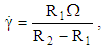 | (44) |
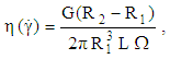 | (45) |
 . Therefore, the viscosity expression
  for this geometry must be corrected to the following form [46]:
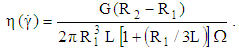 | (46) |
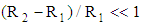
 | Figure 5. Schematic representation for installation method of the rheometer in magnetic field (side view), where N and S are electromagnet poles Bx and Bz are the magnetic field intensity in x– and z–directions respectively |
 and field lines directed perpendicularly to the rotational axis of a rotor.§ the second magnet, with an intensity of
  and field lines parallel to the axis of rotor rotation. The working unit with a solution was placed into the magnetic field at
  and kept for 20min, then the viscosity in the presence of the magnetic field were measured at an increasing shear rate from 0 to
  . During magnetic field application, the solution viscosity grows as a result of orientation of chains molecules under a magnetic field in parallel with the line of force. The magnetic field components are
 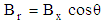 and
and  imposed in r–and z–directions respectively. The, processes occurring during the flow of solutions in the presence of a magnetic field may be represented with the help of Fig. 5 as the following:§ In quadrant I, field lines are parallel to the rotational axis, Fig. 5b. The orientation of molecules chains and the flow direction coincide with opposite directions. In this case, the viscosity may decrease
 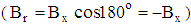 .§ In quadrant III, field lines are parallel to the rotation axis. The orientation of molecules chains and the flow direction are coincides and are in same directions. In this case, the viscosity may increase
 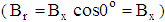 .§ In quadrant II, molecules chains are oriented perpendicularly to the flow direction
 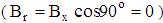 . Therefore, the viscosity remains unchanged.§ In quadrant IV, molecules chains are oriented perpendicularly to the flow direction
 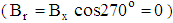 and again the viscosity remains unchanged.§ When the magnetic lines are parallel to the rotational axis,
  in Fig. 5c, the molecules chains are oriented along the axis of rotation, that is, perpendicularly to the flow direction. As a result, viscosity may increase. Lu et al. [39] measured the viscosity of the CNC aqueous suspensions on an AR–G2 rheometer (TA Instruments, USA). The measurements are taken in the shear rate ranging from 0.01 to
  . Temperature control was established with a Thermo–Cube kept within
  of the desired temperature. Shafiei et al. [40] carried out the viscosity measurements on a rotational rheometer (MCR 501 Anton Paar Physica) with parallel flat stainless steel plate geometry of 50nm in diameter and 1nm gap. All rheological measurements were performed at temperature of 298K. Then to describe the flow property, steady state shear viscosity was monitored by increasing the shear rate
  from 0.01 to
  .
. 6. Results and Discussion
6.1. Cellulose Derivatives Flow Curves
- In this section fitting results of the experimental data given in [26-30] and [39, 40] are overviewed to give a coherent picture about the rheological behaviors of the considered solutions and suspensions. Four sets of cellulose derivatives experimental data were used in order to describe their rheological behavior, see Table 3. A good fit for the experimental flow curves can be obtained starting from the understanding the effects of the Giesekus parameters on the flow curve under consideration and finding the proper values for these parameters. Then by inserting the proper values in the Giesekus model explained above we can draw a theoretical curves. The proper parameters values must able the theoretical curve to catch the experimental points. Giesekus model contains four parameters: the zero shear rate viscosity
 , the retardation time
  , the relaxation time
  and the shape factor (a). The suitable values of the four Giesekus parameters required for the best fit are listed in Table 3 for each cellulose derivative with its suitable solvents.
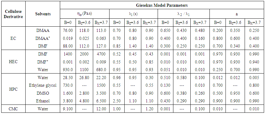 | Table 3. Proper Parameters of Giesekus Model for Cellulose Derivatives and Their Suitable Solvents |
 and the other in z–direction
  to various suspensions and measured their viscosity. During analysis of the viscosity data, we must taken into account that the viscosity is affected by shear rate and the applied magnetic field. As we have seen above, the viscosity of all samples decreases with increasing shear rate and increases with increasing the applied magnetic field. Figures 6 to 9 show flow curves for all used solutions in the presence and in the absence of the magnetic field. In low concentration solutions, molecules chains are few and the field effect is insignificant. The number of molecules capable of orientation in the magnetic field increases with the polymer concentration, and the field effect on the system properties becomes stronger. The increase in solutions viscosity with concentration is related to an increasing number of magnetically sensitive molecular chains. However, at high concentrations, the number of entanglements network increases and begins to hinder the orientation processes and the influence of the field on viscosity of solutions decreases.
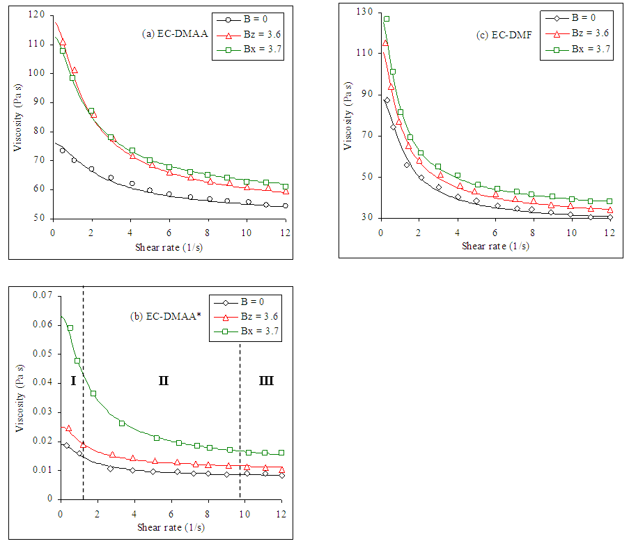 | Figure 6. Viscosity–shear rate curves for EC solutions in (a) DMAA C = 0.25 wt%, (b) DMAA* C = 0.3 wt% and (c) DMF C = 0.25 wt% at different values of magnetic field where dots represent the experimental data taken from [26, 28, 29] and solid lines represent Giesekus model fit |
 | Figure 7. Viscosity–shear rate curves for HEC solutions in (a) DMF C = 0.15 wt%, (b) DMF* C = 0.15 wt% and (c) water C = 0.10 wt% at different values of magnetic field where dots represent the experimental data taken from [26, 28, 26] and solid lines represent Giesekus model fit |
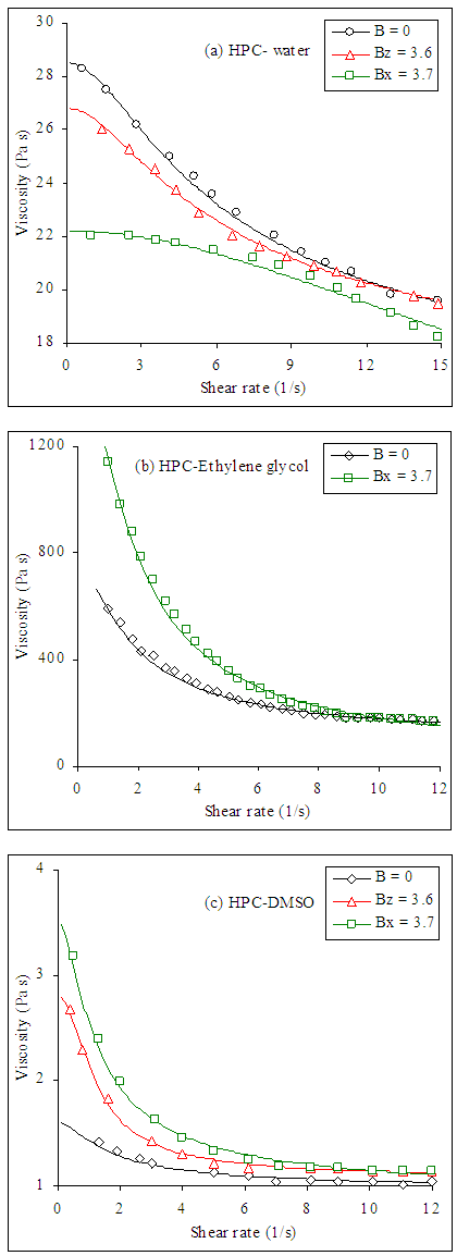 | Figure 8. Viscosity–shear rate curves for HPC solutions in (a) water C = 0.10 wt%, (b) Ethylene glycol C = 0.15 wt%, (c) DMSO C = 0.10 wt% at different values of magnetic field where dots represent the experimental data taken from [26, 29, 30] and solid lines represent Giesekus model fit |
 | Figure 8. (d) Viscosity–shear rate curves for HPC solutions in Ethanol C = 0.41 wt% at different values of magnetic field where dots represent the experimental data taken from [30] and solid lines represent Giesekus model fit |
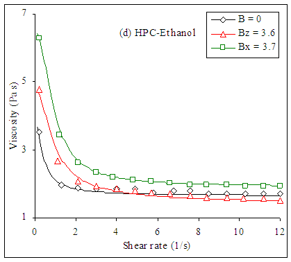
 | Figure 9. Viscosity–shear rate curves for CMC solutions in water C = 0.04 wt% at different values of magnetic field where dots represent the experimental data taken from [27] and solid lines represent Giesekus model fit |
6.2. Relaxation Character of Cellulose Derivatives Viscosity
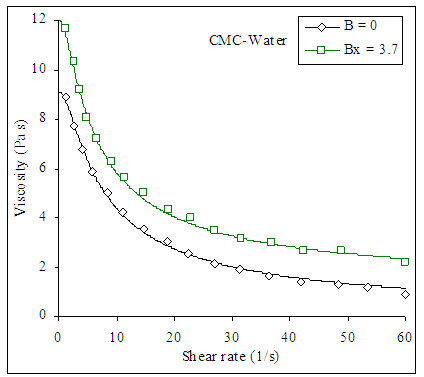
- To investigate the relaxation character of the viscosity behavior of cellulose derivatives solutions, Vshivkov et al. measured the solutions viscosities via two steps, shear rate was increased from 0 to 13s-1 for 10 min (loading) and at the second step, the shear rate was decreased from 13 to 0 s-1 for 10 min (unloading). Figure 10a show the two successive steps of determination the viscosity values of HPC–Ethylene glycol system during loading (filled symbols) and unloading (open symbols) in the absence of the magnetic field. By using the same sample, the loading and unloading curves do not coincide; i.e., a hysteresis loop is observed. Clearly higher viscosities for the increasing shear rate experiments are observed at low shear rates. In fact, when a test is performed the structure network of the HPC solutions is gradually destroyed as the shear rate increases. Hence, in the second experiments conducted from decreasing shear rates on the same sample, lower viscosity values are observed. From this behavior, it can be concluded that the network broken down in increasing shear test cannot be reformed with the same strength in decreasing shear test. Similar results were obtained for more concentrated HPC solutions. As shown in Fig. 10b, the application of a magnetic field results in increased viscosity values and, hence, relaxation times.
 | Figure 10. Viscosity–shear rate curves for HPC solution in ethylene glycol C = 0.15 wt% for increasing and decreasing shear rate and in (a) the absence of magnetic field (B = 0) and (b) at Bx = 3.7 where dots represent the experimental data taken from [29] and solid lines represent Giesekus model fit |
6.3. CNC Suspensions Flow Curves
- To study the effects of shear rate on the rheological behavior of dilute aqueous CNC suspensions, data measured by Lu et al. [39] and Shafiei et al. [40] are considered. The dependence of the viscosity of CNC suspensions on shear rate as measured by Lu et al. can be seen in Fig. 11a. Data are obtained at 298K and at different values of concentrations. The range of shear rate is sufficient to cover the regions in which the viscosities at high shear rates arise to some constant values. In the range of low and intermediate shear rates, the viscosity is a function of concentration. Similar depends were obtained from that data measured by Shafiei et al. in Fig. 11b. The studied suspensions are non–Newtonian fluids, the viscosity decreases when the shear rate increases, a situations that indicates the breaking of the initial structures of polymer suspensions and the orientation of fibers along the flow direction during deformation. The velocity drops significantly and its profile changes to one exhibiting three discrete regions as the following:§ Region I in which the velocity profile consists of a shear thinning at low shear rate due to the alignment of the CNC fibers.§ Region II at intermediate shear rates, where the fibers have continuous alignment and oriented along the shear direction.§ Region III at high shear rates, where the shear stress is high enough to destroy the liquid domains into individual fibers and orient them along the flow direction.According to Fig. 11, although the decrease in viscosity becomes level off at low concentrations, it still significant in the first shear thinning region of the viscosity profiles. The Giesekus model parameters for dilute aqueous CNC suspensions are given in Table 4.
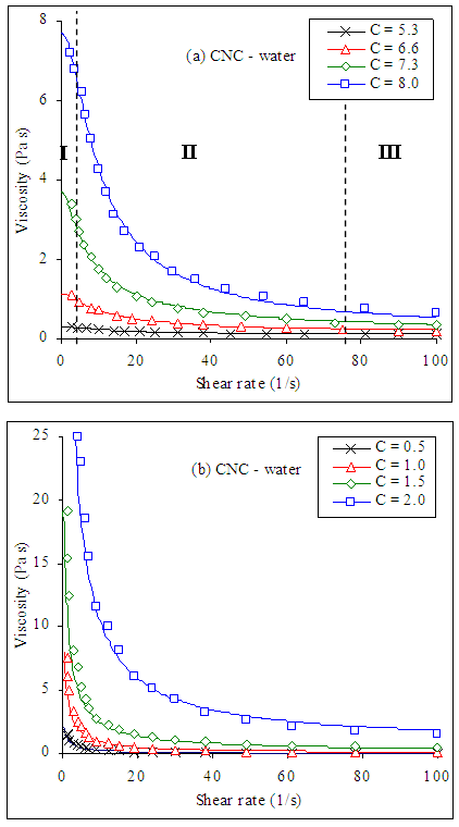 | Figure 11. Viscosity–shear rate curves for CNC aqueous suspensions at different concentrations where dots represent the experimental data taken from (a) Lu et al. [39] and (b) Shafiei et al. [40] and solid lines represent Giesekus model fit |
|
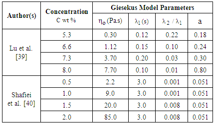
 . The interaction between CNC fibers leads to increased η as the CNC concentration increased. For all samples studied by Lu et al. [39] and Shafiei et al. [40], the viscosity of these suspensions possesses viscoelastic shear thinning characteristics. This shear thinning behavior is due to break down of NCN bond network under the application of shear and the alignment of individual CNC fibers in the direction of shear. However, it must be pointed out that the viscosity measured by Shafiei et al., Fig. 11b, at each constants shear rate and concentration are higher than those measured by Lu et al., Fig. 11a. This arises as a result of the difference in the dimensions of CNC fibers during preparation.
6.4. Effect of Concentration on the Viscosity of CNC Suspensions
- The shear rate and viscosity properties of CNC suspensions are now well documented. They can undergo a phase shift from an isotropic to an anisotropic state before gelling. At low concentrations CNC fibers did not interact much with each other. The suspensions were characterized by a Newtonian plateau, where Brownian motion dominates over shear. As the shear increased, the hydrodynamic forces oriented particles under flow, which decreases the viscosity. At higher concentrations, the system become biphasic with both anisotropic and isotropic phases. The relationship between the concentration of CNC suspensions and its viscosity at constant shear rates is shown in Fig.12a. It can be observed that for concentrations up to 1.5wt%, the CNC suspension presented similar behaviors, which is an increase for viscosities with the concentration. For concentration
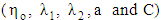
 , there is a sudden increase in viscosity. We can state that the concentration functionality of CNC suspensions is due to the increase in the CNC fibers interactions. Referring to my previous paper [42] we can relate the measured viscosity to shear rate and concentration using the following formula:
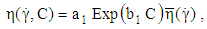 | (47) |
 and
and  are constants. Since Giesekus model accurately predicts the viscosity as a function of shear rate. Hence, the term
  is equivalent to
  in Eq. (13) and the term
  is given by:
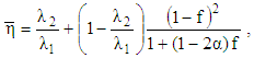 | (48) |
 and
and  are calculated and a new proposed correlation which predict the viscosity of CNC suspensions is:
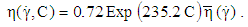 | (49) |
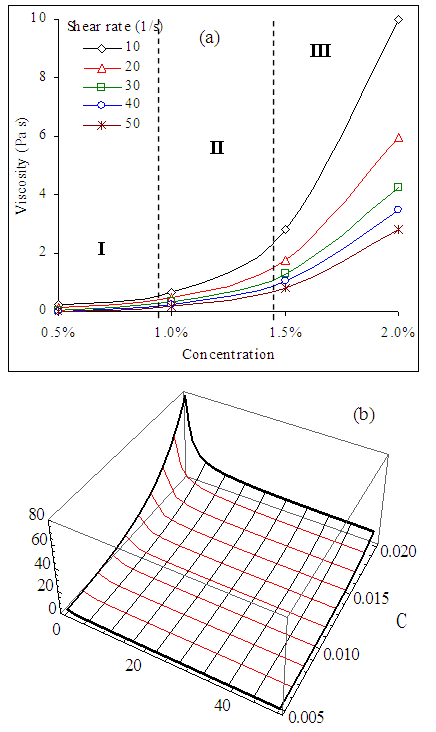 | Figure 12. (a) Concentration dependence of CNC suspension viscosity as calculated in [40] where dots represent the experimental data (b) The combined effects of  and C on η of CNC suspension in 3D and C on η of CNC suspension in 3D |
7. Conclusions
- The objective of this work is to investigate the measured data behaviour of some cellulose derivatives (EC, HEC, HPC and CMC) dissolved in eight acceptable solvents and rheology of dilute aqueous suspensions of cellulose nanocrystals. We reconsider Vshivkov et al. measured data on Rheotest RN 4.1 rheometer for cellulose derivatives at concentrations 0.04, 0.1, 0.15, 0.25, 0.3 and 0.41wt% and Lu et al. and Shafiei et al. measured data on AR–G2 rheometer for CNC suspensions at concentrations 0.5, 1, 1.5, 2, 5.3, 6.6, 7.3 and 8 wt%. The viscosities of the analyzed solutions and suspensions were determined by fitting the data using Giesekus model for viscoelastic polymers. Advantage of using Giesekus model fit is the possibility of carrying out the theoretical analysis for viscosity measurements once an initial parameters have been performed.As seen from the figures, all samples exhibit shear thinning over the whole shear rate range investigated. The effects of magnetic field on rheological properties of cellulose derivatives have been investigated. Polymer viscosity is decreased by increasing the magnetic field strength. This is due to the molecules of cellulose derivatives are characterized by a rigid helical configuration. These molecules orient themselves in the magnetic field so that their long chains are oriented parallel to the magnetic field lines. The CNC suspensions exhibit a similar behavior. At low concentrations (up to 1wt%), the CNC suspensions have a very low viscosity almost independent of the shear rate (Newtonian behaviour ) due to the Brownian motion of the CNC fibers, which prevents them to orient under flow. At very high shear rates, the shear forces tend to orient the fibers along the flow, which leads to a trivial shear thinning of the suspensions. Increasing the concentration above 1wt%, the anisotropic phase appears at low shear rates because the fibers start coming into closer contact. With the help of reported information and illustrated figures, the following conclusions can be deduced:§ The possibility of analyzing the experimental data using Giesekus model supports the fact that this model gives better and more accurate results, as it can be applied in dilute suspensions and polymeric solutions.§ Moreover, the theoretical analysis shows that cellulose derivatives solutions and CNC suspensions are characterized by five parameters
 which must be determined when measuring the flow properties of solutions or suspensions. § A theoretical analysis confirmed that increasing the magnetic field strength decreases the viscosity of the polymeric liquid.§ The viscosity of the solutions with low concentrations showed Newtonian behaviour as the viscosities were not affected by the shear rate. However, by increasing the concentrations the shear thinning behaviour was observed as the viscosity decreased with increased applied shearing stress.§ The drop in viscosity is very sharp as shear rate increases slightly.§ Depending on the concentration, three flow regions are observed. At low concentration, the rheological behaviour simulate a linear relationship (Newtonian fluid) which indicates that the shear rate has less effect on viscosity. While at high concentration, the shear rate has a large effect on viscosity of polymer which simulate the non–Newtonian fluids.§ Final conclusion in this paper is that, the Giesekus model able to describe the rheological properties of any viscoelastic polymer. Before embarking on this description you must first know the values of the model parameters
 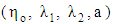 that make the theoretical curve catches the experimental data.
References
| [1] | S. Nishikawa, and S. Ono, Proc. Math. Phys. Soc. Tokyo, vol. 7, pp. 131, 1913. |
| [2] | H. Krässig, Cellulose, Polymer Monographs, vol. 11, Gordon and Breach Science Publishers, Amsterdam, 1996. |
| [3] | F. J. Kolpak, and J. Blackwell, “Determination of the structure of cellulose II,” J. Macromolecules, vol. 9(2), pp. 273–278, 1976. |
| [4] | J. W. S. Hearle, “A fringed fibril theory of structure in crystalline polymers,” J. Polym. Sci., vol. 28(17), pp. 432–435, March 1958. |
| [5] | P. J. Flory, “Statistical thermodynamics of semiflexible chain molecules,” Proc. R. Soc. London, Ser. A, vol. 234, pp. 60, 1956. |
| [6] | R. Werbowy, and D. Gray, Macromolecules, vol. 13, pp. 69, 1980. |
| [7] | R. Werbowy, and D. Gray, Mol. Cryst. Liq. Cryst., vol. 34, pp. 97, 1976. |
| [8] | S. S. L. Tseng, A. Valente, and D. Gray, “Cholesteric liquid crystalline phases based on acetoxypropyl cellulose macromolecules,” vol. 14, pp. 715–719, 1981. |
| [9] | A. M. Ritcey, K. R. Holme, and D. G. Gray, “Cholesteric properties of cellulose acetate and triacetate in trifluoroacetic acid,” Macromolecules, vol. 21, pp. 2914–2917, 1988. |
| [10] | J. X. Guo, and D. Gray, “Preparation and liquid-crystalline properties of (acetyl)(ethyl) cellulose,” Macromolecules, vol. 22, pp. 2082–2086, 1989. |
| [11] | R. Bodvik, A. Dedinaite, L. Karlson, M. Bergström, P. Bäverbäck, J. Skov Pedersen, K. Edwards, G. Karlsson, I. Varga, and P. M. Claesson, “Aggregation and network formation of aqueous methylcellulose and hydroxypropyl methylcellulose solutions,” Colloids and surfaces, series A, vol. 354, pp.162–171, 2010. |
| [12] | H. Boerstel, H. Maatman, J. B. Westerink, and B. M. Koenders, “Liquid crystalline solutions of cellulose in phosphoric acid,” Polymer, vol. 42, pp. 7371–7379, 2001. |
| [13] | S. A. Vshivkov, and E. V. Rusinova, “Liquid crystal phase transitions and rheological properties of cellulose ethers,” Russian Journal of Applied Chemistry, vol. 84(10), pp. 1830–1835, 2011. |
| [14] | P. Zugenmaier, “Materials of cellulose derivatives and fiber–reinforced cellulose–polypropylene composites: characterization and application,” Pure Appl. Chem., vol. 78(10), pp. 1843–1855, 2006. |
| [15] | P. Navard, and J. Haudin, “Rheology of mesomorphic solutions of cellulose,” Br Polym. J., vol. 12(4), pp. 174–178, 1980. |
| [16] | T. Dahl, and A. Kibbe, Hand book of pharmaceutical excipients, American Pharmaceutical Association and Pharmaceutical Press, 2000. |
| [17] | M. Davidovich–Pinhas, S. Barbut, and A. G. Marangoni, “Physical structure and thermal behavior of ethyl cellulose,” Cellulose, vol. 21(5), pp. 3243–3255, 2014. |
| [18] | C. Clasen, and W. M. Kulicke, “Determination of viscoelastic and rheo–optical material functions of water–soluble cellulose derivatives,” Prog. Polym. Sci., vol. 26(9), pp. 839, 2001. |
| [19] | S. Y. Lin, S. L. Wang, Y. S. Wei, and M. J. Li, “Temperature effect on water desorption from methyl cellulose films studied by thermal FT–IR micro spectroscopy,” Surf. Sci., vol. 601(3), pp. 781–785, 2007. |
| [20] | C. H. Chen, C. C. Tsai, W. Chen, F. L. Mi, H. F. Liang, S. C. Chen, and H. W. Sung, “Novel living cell sheet Harvest system composed of thermo–reversible Methyl cellulose hydrogels,” Biomacromolecules, vol. 7(3), pp. 736–743, 2006. |
| [21] | L. Karlson, Hydrophobically modified polymers–Rheology and Molecular Associations, Lund University, Lund, 2002. |
| [22] | T. Sanz, M. A. Fernandez, A. Salvador, J. Munoz, and S. M. Fiszman, “Thermogelation properties of methyl cellulose (MC) and their effect on a batter formula,” Food Hydrocolloids, vol. 19(1), pp. 141–147, 2005. |
| [23] | N. Gowariker, Viswanathan, and J. Sreedhar, Polymer Science, John Wiley and Sons, 1986. |
| [24] | D. Gray, and H. Darley, Composition and properties of oil well drilling fluids, 4th ed., Gulf Publication Co., Houston, 1981. |
| [25] | S. A. Vshivkov, Phase transitions of polymer systems in external fields, Lan. Sankt–Peterburg, 2013. |
| [26] | S. A. Vshivkov, E. V. Rusinova, and A. G. Galyas, “Phase diagrams and rheological properties of cellulose ether solutions in magnetic field,” Eur. Polym. J., vol. 59, pp. 326–332, 2014. |
| [27] | S. A. Vshivkov, and A. A. Byzov, “Phase equilibrium, structure, and rheological properties of the carboxymethyl cellulose–water system,” Polym. Sci., Ser. A, vol. 55(2), pp. 102–106, 2013. |
| [28] | S. A. Vshivkov, E. V. Rusinova, and A. G. Galyas, “Effect of a magnetic field on the rheological properties of cellulose ether solutions,” Polym. Sci A, vol. 54(11), pp. 827–832, 2012. |
| [29] | S. A. Vshivkov, and T. S. Soliman, “Phase Transitions, structures, and rheological properties of hydroxypropyl cellulose–ethylene glycol and ethyl cellulose–dimethyl formamide systems in the presence and in the absence of a magnetic field,” Polym. Sci., series A, vol. 58(4), pp. 499–505, 2016. |
| [30] | S. A. Vshivkov, and T. S. Soliman, “Effect of a magnetic field on the rheological properties of the systems hydroxypropyl cellulose-ethanol and hydroxypropyl cellulose-dimethylsulfoxide,” Polym. Sci., series A, vol. 58(3), pp. 307–314, 2016. |
| [31] | X. M. Dong, T. Kimura, J. F. Revol, and D. G. Gray, “Effects of ionic strength on the isotropic–chiral nematic phase transition of suspensions of cellulose crystallites,” Langmuir, vol. 12(8), pp. 2076–2082, 1996. |
| [32] | Y. Habibi, L. A. Lucia, and O. J. Rojas, “Cellulose nanocrystals: chemistry, self–assembly, and applications,” Chem. Rev., vol. 110(6), pp.3479–3500, 2010. |
| [33] | R. J. Moon, A. Martini, J. Nairn, J. Simonsen, and J. Youngblood, “Cellulose nanomaterials review: structure, properties and nanocomposites,” Chem. Soc. Rev., vol. 40(7), pp. 3941–3994, 2011. |
| [34] | M. Bercea, and P. Navard, “Shear dynamics of aqueous suspensions of cellulose whiskers,” Macromolecules, vol. 33(16), pp. 6011–6016, 2000. |
| [35] | E. Lasseuguette, D. Roux, and Y. Nishiyama, “Rheological properties of microfibrillar suspension of TEMPO–oxidized pulp,” Cellulose, vol. 15(3), pp. 425–433, 2008. |
| [36] | G. Agoda–Tandjawa, S. Durand, S. Berot, C. Blassel, C. Gaillard, C. Garnier, and J. L. Doublier, “Rheological characterization of microfibrillated cellulose suspensions after freezing,” Carbohydr Polym., vol. 80(3), pp. 677–686, (2010). |
| [37] | M. Bercea, and P. Navard, “Shear dynamics of aqueous suspensions of cellulose whiskers,” Macromolecules, vol. 33(16), pp. 6011–6016, 2000. |
| [38] | E. E. Urena–Benavides, G. Ao, V. A. Davis, and C. L. Kitchens, “Rheology and phase behavior of lyotropic cellulose nanocrystal suspensions,” Macromolecules, vol. 44(22), pp. 8990–8998, 2011. |
| [39] | A. Lu, U. Hemraz, Z. Khalili and Y. Boluk, “Unique viscoelastic behaviors of colloidal nanocrystalline cellulose aqueous suspensions,” Cellulose, vol. 21, pp. 1239–1250, 2014. |
| [40] | S. Shafiei–Sabet, M. Martinez, and J. Olson, “Shear rheology of micro–fibrillar cellulose aqueous suspensions,” Cellulose, vol. 23, pp. 2943–2953, 2016. |
| [41] | S. E. E. Hamza, “A comparison of rheological models and experimental data of Metallocene linear low density Polyethylene solutions as a function of temperature and concentration,” Journal of advances in physics, vol. 12(3), pp. 4322–4339, 2016. |
| [42] | S. E. E. Hamza, “Modelling the effect of concentration on non–Newtonian apparent viscosity of an aqueous Polyacrylamide solution,” Global Journal of Physics, vol. 5(1), pp. 505–517, 2016. |
| [43] | S. G. Advani, and C. L. Tucker, “Closure approximations for three dimensional structure tensors,” J. Rheol., vol. 34(3). pp 367–386, 1990. |
| [44] | H. Giesekus, “Stressing behavior in simple shear flow as predicted by a new constitutive model for polymer fluids,” J. Non–Newtonian Fluid Mech., vol. 12, pp. 367–374, 1983. |
| [45] | H. Giesekus, “A simple constitutive equation for polymer fluids based on the concept of deformation dependent tensorial mobility,” J. Non–Newtonian Fluid Mech., vol. 11, pp. 69–109, 1982. |
| [46] | R. B. Bird, C. F. Curtiss, R. C. Armstrong, and O. Hassager, Dynamics of Polymeric Liquids, 2nd ed., vol. 2, Kinetic Theory, Wiley Interscience, New York, 1987. |
| [47] | V. N. Kalashnikov, “Shear rate dependent viscosity of dilute polymer solutions,” J. Rheol., vol. 38(5), pp. 1385–1403, 1994. |
| [48] | W. Pabst, “Fundamental considerations on suspension rheology,” Ceramics Silikaty, vol. 48(1), pp. 6–13, 2004. |
| [49] | F. Rodriguez, Principles of polymer systems, 2nd ed., McGraw Hill chemical engineering series, 1983. |
| [50] | G. L. Hand, “A theory of dilute suspensions,” Arch. Ration. Mech. Anal., vol. 7, pp. 81–86, 1961. |
| [51] | C. Crowe, “Review numerical models for dilute gas particles flow,” J. Fluids Eng., Tran. ASME, vol. 104, pp. 297–303, 1982. |
| [52] | S. G. Advani, and E. M. Sozer, Process modeling in composites manufacturing, Marcel Dekker Inc., New York, 2003. |
| [53] | G. L. Hand, “A theory of anisotropic fluids,” J. Fluid Mech., vol. 13, pp. 33–62, 1962. |
| [54] | S. E. E. Hamza, “Basic concepts of rigid fiber suspensions rheology,” Global Journal of Physics, vol. 5(2), pp. 562–584, 2017. |
| [55] | S. Onogi, and T. Asada, “Rheology and rheo–optics of polymer liquid crystals,” Rheology, vol. 1, pp 127–147, 1980. |