-
Paper Information
- Paper Submission
-
Journal Information
- About This Journal
- Editorial Board
- Current Issue
- Archive
- Author Guidelines
- Contact Us
American Journal of Fluid Dynamics
p-ISSN: 2168-4707 e-ISSN: 2168-4715
2017; 7(1): 12-22
doi:10.5923/j.ajfd.20170701.02

Preliminary Study of Supersonic Partially Covered Cavity Flow with Scaled Adaptive Simulation
 Abstract
 Reference
 Full-Text PDF
 Full-text HTML
Christopher Teruna, Duck Joo Lee
Department of Aerospace Engineering, KAIST, Daejeon, South Korea
Correspondence to: Christopher Teruna, Department of Aerospace Engineering, KAIST, Daejeon, South Korea.
| Email: |  |
Copyright © 2017 Scientific & Academic Publishing. All Rights Reserved.
This work is licensed under the Creative Commons Attribution International License (CC BY).
http://creativecommons.org/licenses/by/4.0/

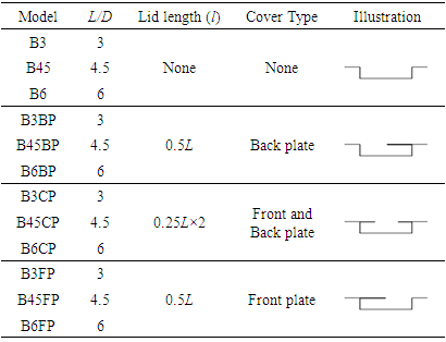
We investigate supersonic flow over rectangular cavities of 3 different length-to-depth ratio (L/D) – 3, 4.5, and 6. Half of the length of the cavities will be covered additional lids of D/d = 6, in which D/d is the ratio of cavity depth to lid thickness. The lids were installed to either leading edge (FP), trailing edge (BP), or both edges (CP) of the cavities, resulting in 12 variety of cavity configurations. Validation study was performed beforehand to ensure the reliability of Scaled Adaptive Simulation (SAS) turbulence model for supersonic cavity flow simulation in 2-dimensional (2D) domain. Subsequently, pressure fluctuation on cavity floor was obtained through numerical simulation on each cavity model and its frequency response was analysed. The use of partial cover was found to shorten the length of shear layer, which in turn caused mode switching in dominant cavity tones and various changes in mean pressure distribution. Furthermore, certain flowfield characteristics of partially covered cavities were also identified, depending on partial cover configuration and cavity length. These characteristics are also similar to those previously observed in subsonic partially covered cavity flow.
Keywords: Cavity flow, Scale adaptive simulation, CFX, Frequency response, Pressure distribution
Cite this paper: Christopher Teruna, Duck Joo Lee, Preliminary Study of Supersonic Partially Covered Cavity Flow with Scaled Adaptive Simulation, American Journal of Fluid Dynamics, Vol. 7 No. 1, 2017, pp. 12-22. doi: 10.5923/j.ajfd.20170701.02.
Article Outline
1. Introduction
- The study of cavity flow has always been one of the most intriguing topics among fluid dynamics scholars since it involves various physical attributes, such as aerodynamics and acoustics. Early studies, notably by Karamcheti [1] and Rossiter [2] found that high speed flow over cavity would produce self-sustaining pressure fluctuation inside the cavity and sound radiation away from it. The frequency domain of the pressure fluctuation has several discrete peaks that possess most energy in the spectra, and were subsequently referred to as cavity tones. Rossiter also revealed that cavity tones are products of a feedback mechanism that involved both fluid and acoustic physics that originated from the shear layer spanning across the cavity due to velocity difference between high velocity freestream and stagnant flow inside the cavity. The shear layer, which evolved from upstream boundary layer, is “flapping” upward and downward periodically, and at some point, impinges on the cavity’s aft wall (also referred to as trailing edge in Figure 1). This impingement produces acoustic wave that will propagate upstream along the cavity floor. As these waves arrive at the cavity’s front wall, they would excite and subsequently produce more instabilities in the newly developed shear layer at the cavity’s leading edge. Thus, the system forms a close loop between fluid and acoustic interactions surrounding the cavity.
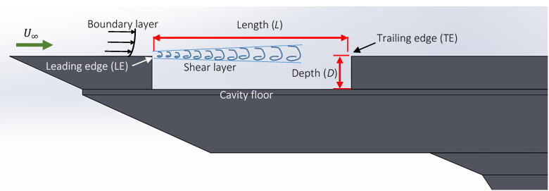 | Figure 1. Nomenclature of cavity flow in this paper |
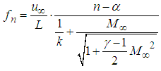 | (1) |
2. Methodologies
2.1. Numerical Setup
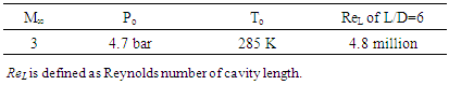
- Since this numerical study would be a precursor to experimental campaign, the numerical setup will be based on experimental equipment which is briefly discussed here. Experiments will be carried out in ST-15 supersonic wind tunnel of High Speed Laboratory of Delft University of Technology. The chosen freestream flow conditions can be found in table 1. The blow-down wind tunnel is operable within Mach number of 1.5 – 3.0 by using suitable nozzle and adjusting total pressure (Po). Total temperature (To) depends on air temperature in pressurized air tank that is placed outdoor and thus variations are affected by daily outdoor air temperature. Therefore, small variations in operating condition might exist but were neglected in numerical simulation.
|
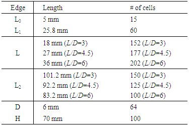
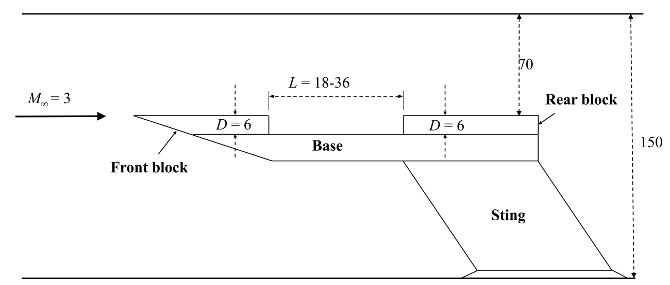 | Figure 2. Side view of cavity model used in present study, dimensions are given in millimetres (mm) |
|
|
 | Figure 3. 2-D computational domain for present study |
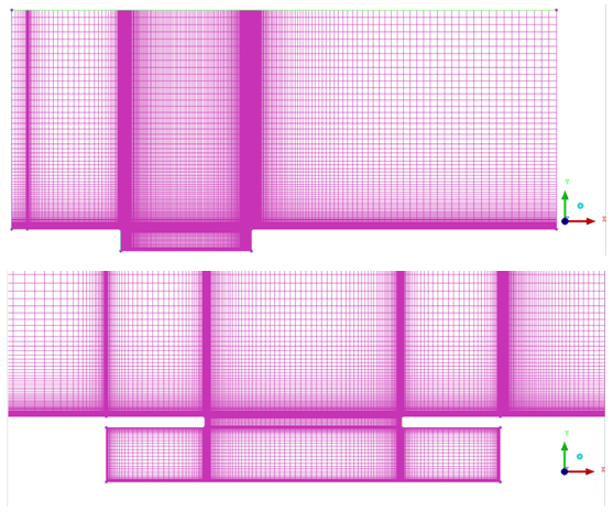 | Figure 4. Mesh generated with ICEM CFD: whole domain of B6 (above) and a close up mesh near B6CP cavity (below) |
2.2. Scaled Adaptive Simulation
- This section will briefly introduce SAS-SST turbulence model that is applied in ANSYS CFX. More in-depth details of SAS and its implementation in CFX can be found in [12], [13], and [14].SAS is an improvement over conventional k-ω model – which is a RANS model, by introducing von Karman length scale in the turbulence scale equation. This allows SAS to adapt resolved turbulent spectrum according to unsteadiness in the flowfield. Practically, SAS is applied as additional source term QSAS in turbulence dissipation equation, ω. To elaborate, k-ω-SST equations with QSAS in ANSYS CFX are given as follows:
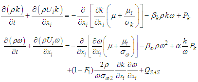 | (2) |
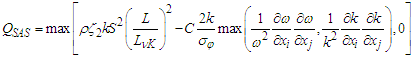 | (3) |
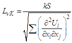
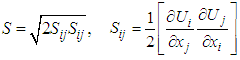
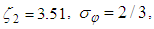 and C = 2. Meanwhile, L is the length scale of modelled turbulence,
  is von Karman length scale, which is generalized from its boundary layer definition, and S is scalar invariant of strain rate tensor Sij.
 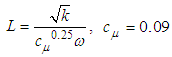 | (4) |
 | (5) |
 | (6) |
3. CFX 2D Validation Study
- While supersonic cavity flowfield is inherently 3-dimensional (3D), it is also interesting to find out if 2-dimensional (2D) simulation would still be adequate (in fact, Rossiter equation is 1-dimensional). After all, parametric analysis for engineering purposes would involve numerous simulations and computing 2D domain would require much lower computational load. However, 2D simulation might produce results with lower accuracy since turbulent flow is inherently 3-dimensional. This validation study will scrutinize the efficacy of 2D-SAS cavity flow simulation.
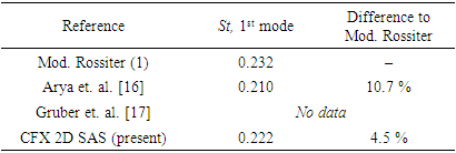
3.1. Cavity Tones of Mach 2 Supersonic Cavity Flow
- This simulation is based on Zhuang’s [15] cavity with L/D of 5.2 and L/W of 5.92 which implies that the cavity is 3-dimensional. Computational domain modelling is similar to Figure 3 except now the cavity is 122 mm long, 23.6 mm deep, and 20.5 mm wide. Inlet flow condition is Mach 2 and u∞ = 548 m/s.Frequencies predicted using Rossiter equation, up to mode 6, is plotted in Figure 5 as vertical dashed line with the mode number printed near the horizontal axis. While cavity tone frequencies seemed to be in good agreement, yet there are discrepancies in amplitude, which is defined as sound pressure level (SPL). SPL itself is defined as logarithmic measure of pressure relative to reference value of 20 µPa (threshold of human hearing) in (7).
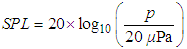 | (7) |
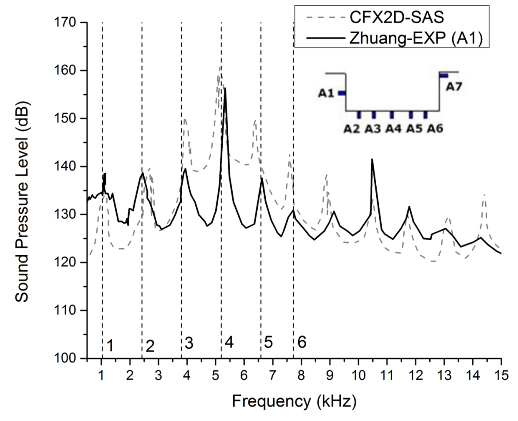 | Figure 5. Frequency response of pressure fluctuation at cavity’s front wall in Mach 2 supersonic cavity flow |
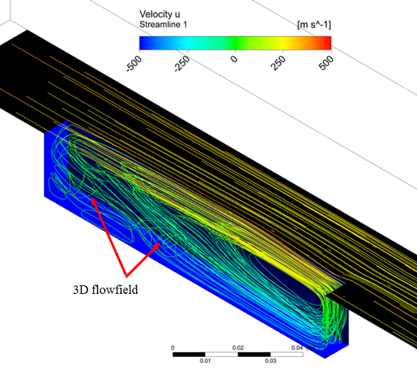 | Figure 6. Streamlie of Zhuang’s cavity simulation with CFX-SAS. The cavity domain is cut along lengthwise symmetry in this figure |
3.2. Cavity Floor Pressure Distribution at Mach 3
- The second case is a comparison of mean pressure distribution along cavity floor. There are two references for comparison: 1) LES simulation with OpenFOAM by Arya et al. [16] and 2) experimental and k-ω simulation results by Gruber et al. [17]. For this case, 2D computational domain was derived from Gruber et al.’s simulation of a cavity with L/D = 3 – identical configuration with B3 cavity.Figure 7 shows that 2D CFX simulation is generally in good agreement with Gruber’s experiment, although overestimation is also detected at the upstream region of the cavity. This overestimation could be related to the similar behaviour of frequency response in Figure 5, but at the moment, no conclusive evidence could be found. Nevertheless, present CFX-SAS results seems to be in good agreement with previous experimental and numerical data obtained by others.
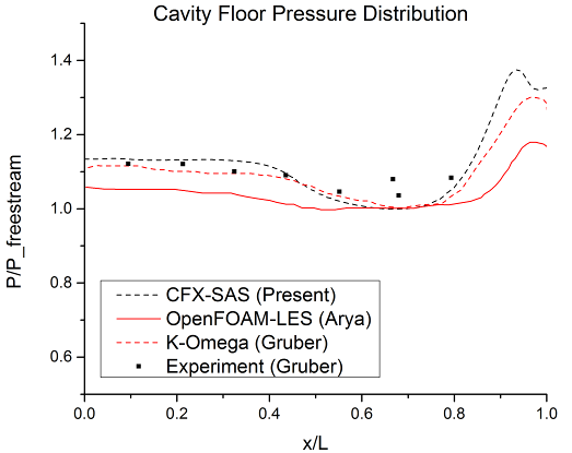 | Figure 7. Comparison of mean pressure distribution along cavity floor, vertical axis is defined as ratio of local pressure to freestream pressure |
|
4. Results and Discussions
4.1. Numerical Results
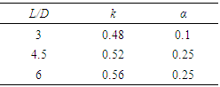
- Frequency domain of pressure fluctuation on cavity floor from CFX simulation is shown in Figure 9 where it is arranged according to each model name. For the case of baseline cavity (B3, B45, and B6), tone frequencies (roman numbers) were found to correspond to Rossiter frequencies (i.e. 17.5 kHz of Rossiter mode IV for B6) that were obtained using (1). Although k = 0.57 α = 0.25 are used typically, but the values that provided better fit are given in Table 5. Comparison between cavity tones of baseline cavities and those from Rossiter equation is given in Figure 8.
|
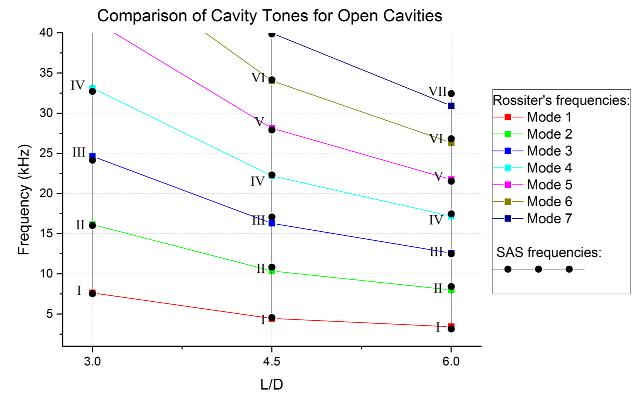 | Figure 8. Baseline cavity (B3, B45, and B6) tone frequency comparison to Rossiter equation. Roman numbers correspond to those in Figure 8 |
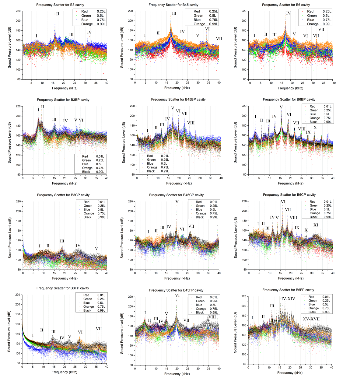 | Figure 9. Frequency responses of pressure fluctuation on cavity floor of all cavity models |
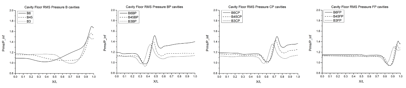 | Figure 10. Root-mean-square (RMS) average of pressure distribution along cavity floor, rearranged based on cover/lid configuration. Vertical axis is defined as ratio of local pressure to freestream pressure |
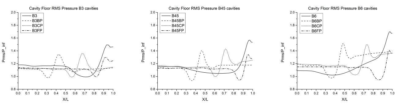 | Figure 11. Root-mean-square (RMS) average of pressure distribution along cavity floor, rearranged based on cavity length. Vertical axis is defined as ratio of local pressure to freestream pressure |
 | Figure 12. Averaged streamlines and velocity contours |
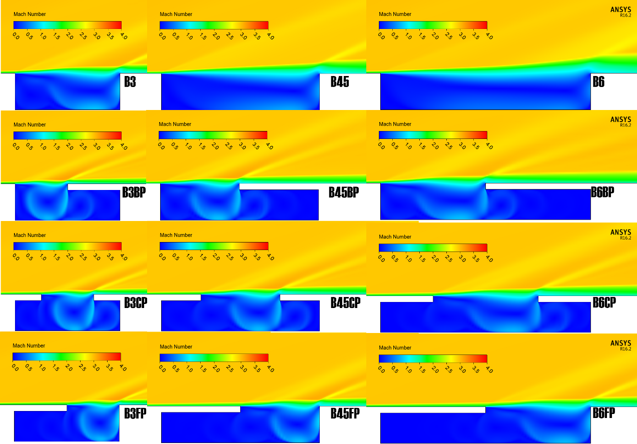 | Figure 13. Averaged Mach number contours |
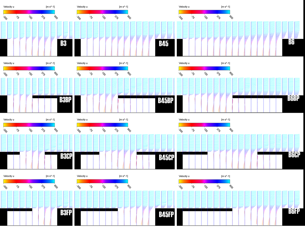 | Figure 14. Averaged velocity vector contours |
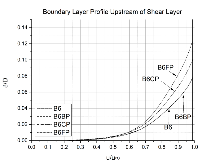 | Figure 15. Comparison of velocity profile upstream of shear layer separation. Vertical axis is defined as ratio of boundary layer thickness and cavity depth |
4.2. Applications of Partially covered Cavities
- Present study of partially covered cavities also beg a very interesting question: which partial cover configuration exhibit the best overall performance? Unfortunately, there is no definitive or exact answer to it, since the term “best performance” here could vary from different perspectives.Based on acoustic performance, i.e. lower pressure fluctuation, either CP or FP configuration would be preferable as both reduce overall SPL level compared to BP and baseline configurations. FP cavity in subsonic flow, in fact, has been widely applied for nose landing gear bay and door mechanism [9]. CP configuration is also applicable for landing gear door, since it resembles that of Helmholtz resonator, i.e. muffler, which was found to reduce noise of certain range of frequency.Meanwhile, BP cavities may be beneficial for high-speed combustion systems, such as ramjet flame-holder. When designing such systems, flow instabilities produced by cavities would enhance fuel-air mixing process. In the case of BP configuration, RCRs inside the cavity were found to be more energetic, i.e. higher flow velocity underneath the cover, compared to other configurations. Therefore, BP cavity may offer an improvement in flame-holding capability of present cavity-based combustors.Overall, each cavity configuration possesses different characteristics that would be favourable for different purposes. However, present study did not account for aero-elastic response of the partial cover, which could have a significant influence to the performance of each cavity configuration. Therefore, future investigations into the application of partially covered cavity are still intriguing nonetheless.
5. Conclusions and Outlooks
- This paper presents a preliminary study of supersonic flow over various partially covered cavities using Scaled Adaptive Simulation (SAS) in ANSYS CFX which was developed by Egorov and Menter [12, 13]. At first, validation study was performed to assess the efficacy of SAS turbulence model for supersonic cavity flow. The study showed good agreement for pressure distribution on cavity floor; although there was overestimation in sound pressure level (SPL) of frequency response. Similarly, Das and Kurian [19], Hamed et. al. [20] and Nayyar et. al. [21] found that pressure oscillation from 2D simulations of cavity whose L/W > 1 would overestimate experimental results while cavity tone frequencies were still resolved within reasonable accuracy.Subsequently, SAS turbulence model was applied for the simulations of 12 cavity configurations. Baseline cavity tones from SAS were in good agreement with frequencies from Rossiter equation. Frequency responses of partially covered cavities were significantly different to those of baseline cavities. However, certain behaviours such as mode switching of dominant cavity tones were observed. Thus, it is surmised that supersonic partially covered cavity flow is sharing some physical similarities with its subsonic counterpart.Undoubtedly, doors for future studies are still wide open, especially since present work only accounts for a few variable parameters. Future parametric studies, by accounting variation of d/D, l/L or the geometry of the lid itself, will be required to formulate prediction models of arbitrary partially covered cavities. It is also envisaged that high-accuracy scheme is required to fully resolve acoustic field inside the partially covered cavity that has been overlooked in present work.
ACKNOWLEDGEMENTS
- This study is a part of an ongoing research collaboration between KAIST (South Korea) and Delft University of Technology (The Netherlands). The author would like to acknowledge both universities for providing grant and support for computational facilities.