-
Paper Information
- Paper Submission
-
Journal Information
- About This Journal
- Editorial Board
- Current Issue
- Archive
- Author Guidelines
- Contact Us
American Journal of Fluid Dynamics
p-ISSN: 2168-4707 e-ISSN: 2168-4715
2016; 6(2): 42-50
doi:10.5923/j.ajfd.20160602.02

Anisotropic Diffusion for Filtering of Forced Homogeneous Isotropic Turbulence
 Abstract
 Reference
 Full-Text PDF
 Full-text HTML
Waleed Abdel Kareem 1, Mahmoud Abdel Aty 2, Zafer M. Asker 1
1Department of Mathematics and Computer Science, Faculty of Science, Suez University, Suez, Egypt
2Department of Mathematics, Faculty of Science, Benha University, Benha, Egypt
Correspondence to: Waleed Abdel Kareem , Department of Mathematics and Computer Science, Faculty of Science, Suez University, Suez, Egypt.
| Email: |  |
Copyright © 2016 Scientific & Academic Publishing. All Rights Reserved.
This work is licensed under the Creative Commons Attribution International License (CC BY).
http://creativecommons.org/licenses/by/4.0/

The anisotropic diffusion model (ADM) that proposed for noise removal of band-pass signals is developed to a three dimensional model to decompose forced homogeneous turbulence into coherent and incoherent parts. The incoherent part represents the noisy data in the flow field, however the coherent part represents the important data for turbulence studies. The velocity flow field is generated by the Lattice Boltzmann method with resolutions of 1283 and 2563 grid points, respectively. The high rotational method, namely the Q-identifying method, is used to identify the vortical structures. The scalar tensor Q is the second invariant of the velocity gradient tensor  The ADM filtering model is applied against the scalar field Q. Results show that the model is a promising tool for fluid dynamics applications. The method identifies the coherent vortices with similar geometrical shapes to the vortices in the original field. The proposed filtering method also isolates the non-organized structureless regions successfully.
Keywords: Complex anisotropic diffusion, Lattice Boltzmann, Coherent and incoherent flows
Cite this paper: Waleed Abdel Kareem , Mahmoud Abdel Aty , Zafer M. Asker , Anisotropic Diffusion for Filtering of Forced Homogeneous Isotropic Turbulence, American Journal of Fluid Dynamics, Vol. 6 No. 2, 2016, pp. 42-50. doi: 10.5923/j.ajfd.20160602.02.
Article Outline
1. Introduction
- The phenomenon of turbulence was discovered physically and is still largely need to explore by mathematical techniques. The analysis of turbulent flow field is too much complicated than that of laminar flows. So, extraction and filtering of homogeneous isotropic turbulence are important processes. The extraction process depends on identifying different scales of the flow, however the filtering process divides the fluid flow field into the coherent and incoherent parts. Most of filtering methods for turbulent problems are applied using the frequency analysis such as the wavelet and Fourier decompositions. These methods are applied against 2D and 3D velocity fields to extract the organized coherent and the random incoherent fields. Wavelets method has significantly impacted many areas of science and engineering (e.g., signal and image processing, speech recognition, and computer graphics). This unification has its own dynamics, allowing scientific cooperation between researchers from very various fields and modifying deeply the scientific perception of many issues in each of these fields. In fluid mechanics, wavelets were first used in the early 1990s, almost since their invention, to analyze the structure and dynamics of two dimensional flow (M. Farge. [1], M. Farge et al. [2], [3], [4], M. Farge and G. Rabreau [5]). For instance the extraction of the coherent vortices from turbulent flows, using the wavelet filtering techniques was discussed by K. Schneider et al. [6], [7] and K. Yoshimatsu et al. [8]. A wavelet nonlinear filtering method for extraction coherent vortices out of hydrodynamic turbulent fields, called coherent vortex extraction (CVE) method is based on a wavelet decomposition of the vorticity field (M. Farge et al. [9] and M. O. Domingues et al. [10]). The method is used in three-dimensional flows using vector-valued wavelet decomposition. The orthogonal and biorthogonal wavelets are compared in [11]. Also the Fourier transform is an integral transform with orthogonal sinusoidal basis functions of different frequencies. In practical implementations of the discrete Fourier transform, it is not used directly but rather a recursive form known as the fast Fourier transform (FFT) is used. K. Schneider et al. [12] compared the CVE method with linear Fourier filtering (LFF), using the spectral cutoff filter. Comparisons of wavelet method with Fourier Nonlinear filtering method were presented by K. Yoshimatsu et al. [8].On the other hand, there are many different methods used in image filtering and they show a high ability in noise reduction. Partial differential equations (PDEs) are one of those methods. PDEs based methods have been applied widely by many researches in image restoration and the other applications like image segmentation, motion analysis and image classification. In Fluid mechanics, (PDEs) transformed the filtering problems to a continuous domain which becomes independent from the grid used in the discrete problem. In image enhancement problems, some PDEs filtering methods focused on parabolic equations. Recently Abdel Kareem [13] examines the ability of (PDEs) to extract coherent and incoherent parts of a turbulent field, where the fourth order (PDEs) are used for the filtering process. Osher and L. Rudin [14], Chan et al. [15], Lysaker et al. [16], and Lysaker and Tai [17] used different PDEs methods for image restoration and filtering. Perona and Malik (PM) [18] in a pioneering work proposed a nonlinear noise removal algorithm of low pass signals and images containing discontinuities, and this model has been extensively studied since it was introduced. The famous Perona-Malik model has been considered as a useful tool for image noise removal and other areas of image processing ([19], [20]). This model could be posed rapidly as a mathematical tool with the great capabilities to image restoring by convolving the original image with a Gaussian kernel. One of the main advantages of the usage of (PDEs) is to take the filtering problems to continuous domain which becomes independent from the grid used in the discrete problem. The Perona and Malik model can preserve edges while removing the noise. However the defect of traditional (PM) model is tending to contain the staircase effect in the processed image.Mahmoodi [21] proposed an algorithm which demonstrates better performance for band pass noisy signals containing discontinuities in comparison with traditional Perona and Malik algorithm. It is important to note that the original (PM) algorithm removes the high frequency component of the original band pass signal, because it behaves like a low pass filter. Therefore Mahmoodi proposed a new method which removes the noise and also preserves discontinuities and high frequency carrier. In this paper, the same Partial differential equation filtering model [21] is developed to a three dimensions model to extract the coherent and incoherent parts of forced homogeneous isotropic turbulent flow fields with resolutions of 1283 and 2563.The paper is organized as follows. Section 1 is the current introduction. In section 2, the characteristics of the anisotropic model in one dimension and its form in 3D will be discussed. In section 3, the important characteristic of the fluid flow and the Lattice Boltzmann method are briefly introduced. Section 4 is devoted to the results of the filtering model. In section 5, the concluding remarks of the study and the future work problems are considered.
2. Characteristics of Anisotropic Diffusion Model
- The anisotropic diffusion model that proposed by Mahmoodi [21] for noise removal is considered to extract coherent and incoherent parts from 3D isotropic turbulent flow fields with resolutions of 1283 and 2563 respectively. First the one dimension model will be discussed. Then the 3D form of the model is derived mathematically. The real and imaginary parts of the model are used in the mathematical derivation.
2.1. One Dimension Anisotropic Diffusion Model
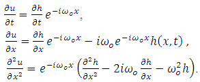
- Let us consider the one dimensional heat equation as
 | (1) |
 where
where  is the smoothed low pass signal at the evolution time
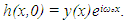
  is the original low pass noisy signal and
  is a constant. Mahmoodi [21] denoted
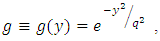
  as a complex valued band pass signal at virtual time t as following
  | (2) |
 | (3) |
 | (4) |
 | (5) |
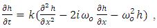
 Equation (5) can be written as
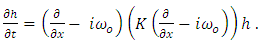 | (6) |
 | (7) |
 | (8) |
 | (9) |
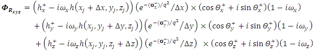
2.2. Three Dimensional Anisotropic Diffusion Model
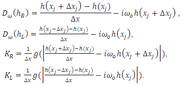
- The ADM in three dimensional form can be written as
 | (10) |
 and consider that
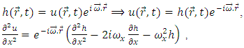 also for z and y directions we find that
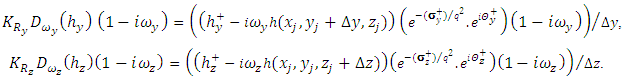
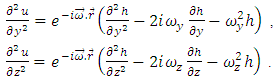 Finally the model in Eqn. (1) can be written in three dimensions as follows
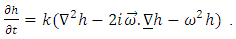 | (11) |
 | (12) |
 | (13) |
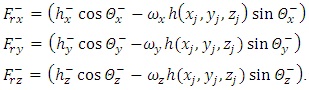
 and
and  are defined as
 | (14) |
 | (15) |
 | (16) |
 | (17) |
 | (18) |
 | (19) |
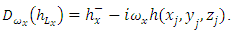
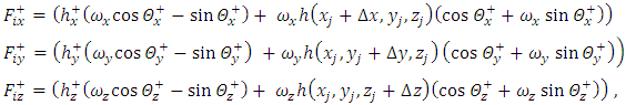
 can be written as follows(1) The first term
 | (20) |
 | (21) |
 | (22) |
 | (23) |
 | (24) |
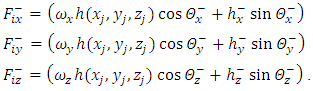
 as follows(1) The first term
 | (25) |
 | (26) |
 | (27) |
 | (28) |
 the following equations are obtained
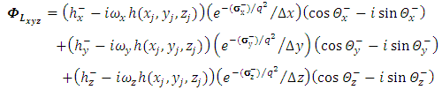 | (29) |
 | (30) |
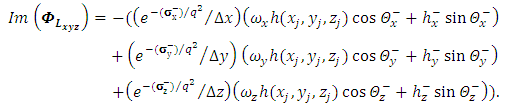
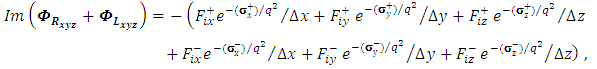
 and
and  to real and imaginary parts, we have
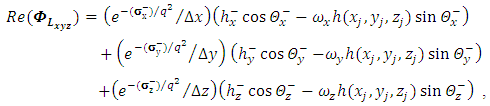 | (31) |
 | (32) |
 we have,
 | (33) |
 | (34) |
 | (35) |
 | (36) |
 | (37) |
 | (38) |
 | (39) |
 | (40) |
3. Simulations and Characteristics of Turbulent Fields
- Recently, the lattice Boltzmann method (LBM) is used as a new computational tool to simulate three dimensional decaying [22] and forced homogenous isotropic turbulence [23]. Abdel Kareem et al. [23] generated the velocity fields of the forced turbulent flow fields using the single relaxation time Lattice Boltzmann model. They used the D3Q19 model to simulate the flow field in a periodic box with a length side of 128. Also, they applied the D3Q15 model to simulate the flow field in a periodic box with a side length of 256. In this study, the obtained velocities of those simulations will be used in the investigation. Here, a brief discussion of the Lattice Boltzmann method will be considered. The lattice Boltzmann equation with a forcing term can be written as
 | (41) |
 represents the additional forcing term. The parameters
  and
and  or
or  are the relaxation time which is related to the fluid viscosity, the discrete velocity set and
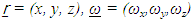
  is an index spanning the momentum space, respectively. More details about the LBM and the used parameters can be found in [23].Some important characteristics of the velocity field can be extracted to describe the features of the simulated turbulent flows. One of those variables is the energy spectrum function E(k) at the scalar wave number
  and it is defined in spectral space by
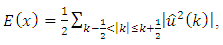 | (42) |
 are the Fourier coefficients. The energy spectrum function E(k) shows the energy transfers from large scales at low wave numbers to the small scales at higher wave number.Also, the second invariant of the velocity gradient tensor, namely Q is defined as [24]
 | (43) |
 symmetric and the antisymmetric components of
  The first term SijSij represents the magnitude of deformation and the second term ΩijΩij represents the magnitude of rotation. This definition will be used in this study to visualize the vortices in all cases (non-filtered fields, coherent fields and incoherent fields). Clearly from the definition positive values of Q identify regions with high rotation where ΩijΩij is dominant.
4. Results and Discussions
4.1. The Non-Filtered Fields
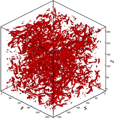
- The non-filtered field that is visualized using the Q-identifying method is shown in Fig. 1 for the 1283 case. The field contains coherent and incoherent parts which cannot be distinguished from each other. The energy spectrum function is shown in Fig. 2 for the 1283 velocity field. Also, Fig. 3 shows the nonfiltered field for the 2563 case and Fig. 4 shows its energy spectrum function. It is clear that more vortices in this case are visualized and the energy spectrum has longer
 slope [25].
 | Figure 1. Isosurfaces of the non-filtered field (resolution  ) ) |
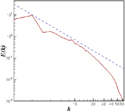 | Figure 2. Energy spectrum (resolution  ) ) |
 | Figure 3. Isosurfaces of the non-filtered field (resolution  ) ) |
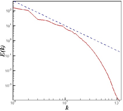 | Figure 4. Energy spectrum (resolution  ) ) |
4.2. ADM Filtering Results
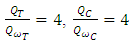
- Before the discussion of the filtering results, the filtering parameters will be discussed. We use the parameters of

 and
and 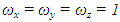 in both 1283 and 2563 data sets. The diffusion constant q is chosen to be 4 in both cases. The criteria for the number of iteration steps in both cases is
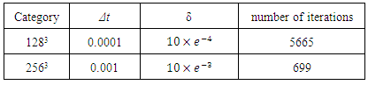
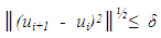 where δ is a small quantity. The parameters δ and Δt are shown in table 1 for the 1283 and 2563 cases.
|
 and
and 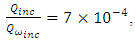 for the 1283, respectively. Here all threshold values are normalized by average entropy
  where
where  is the enstrophy for the coherent data,
  is the enstrophy for the incoherent data and
  is the enstrophy for the non-filtered data.
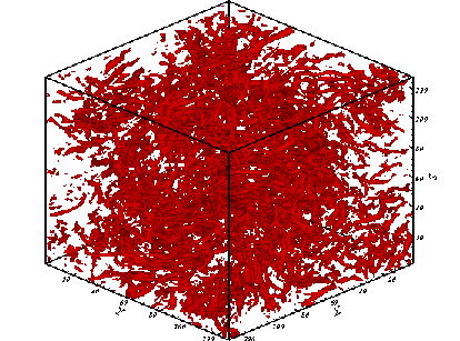 | Figure 5. Isosurfaces of the coherent part (resolution  ) ) |
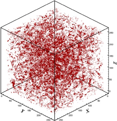
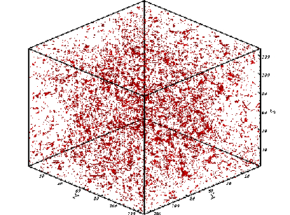 | Figure 6. Isosurfaces of the incoherent part (resolution  ) ) |
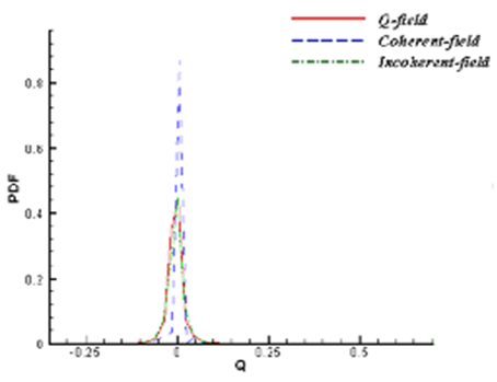
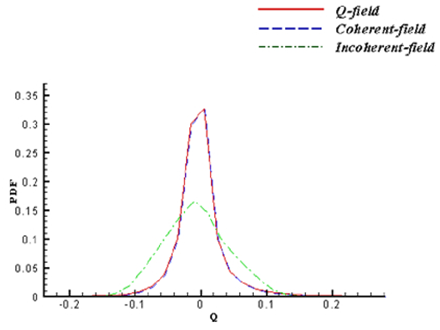 | Figure 7. PDFs of total, coherent and incoherent parts (resolution  ) ) |

 and
and  for the non-filtered field, the coherent field and the incoherent field, respectively.
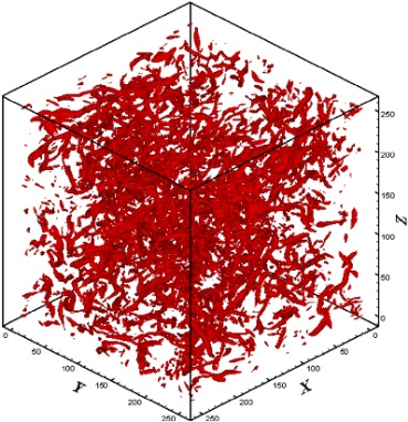 | Figure 8. Isosurfaces of the coherent part (resolution  ) ) |
 | Figure 9. Isosurfaces of the incoherent part (resolution  ) ) |
 | Figure 10. PDFs of total, coherent and incoherent parts (resolution  ) ) |
5. Conclusions
- The one dimensional complex anisotropic diffusion model that proposed for noise removal is developed to a three-dimensional model for filtering of forced turbulent flows into coherent and incoherent parts. The model is found robust in identifying the coherent part with vortices similar in its geometrical shapes as well as their PDF distributions to the original flow field. The incoherent parts are found as structureless regions and they are distributed randomly in the flow field. Identifying the noisy part of the flow field improves the understanding of the dynamics of turbulence and also reduces the time consuming for analysis the huge data of turbulence. There are some important issues that not addressed in the study and they can be considered in future work. Those issues such as extracting the coherent and incoherent flows of the different scales from the flow field using the ADM model and applying the model to higher resolution data sets for different problems in fluid dynamics.