-
Paper Information
- Paper Submission
-
Journal Information
- About This Journal
- Editorial Board
- Current Issue
- Archive
- Author Guidelines
- Contact Us
American Journal of Fluid Dynamics
p-ISSN: 2168-4707 e-ISSN: 2168-4715
2016; 6(2): 27-41
doi:10.5923/j.ajfd.20160602.01

A New Mathematical Approach to the Turbulence Closure Problem
 Abstract
 Reference
 Full-Text PDF
 Full-text HTML
Mohammed A. Azim
Department of Mechanical Engineering, Bangladesh University of Engineering and Technology, Dhaka, Bangladesh
Correspondence to: Mohammed A. Azim, Department of Mechanical Engineering, Bangladesh University of Engineering and Technology, Dhaka, Bangladesh.
| Email: |  |
Copyright © 2016 Scientific & Academic Publishing. All Rights Reserved.
This work is licensed under the Creative Commons Attribution International License (CC BY).
http://creativecommons.org/licenses/by/4.0/

This study introduces a new mathematical approach (NMA) stating that the remaining small terms upon dominant balance, if retains the essential physics of the original equation, may exist as an additional equation. Application of this additional equation appears to reduce the unclosed governing equations for the two-dimensional turbulent flow to closed ones. The closed form equations due to NMA for the turbulent boundary layer and round jet are solved using a Fully Implicit Numerical Scheme and the Tridiagonal Matrix Algorithm. An overall agreement of the obtained results with the existing database for both types of flow show the capability of NMA in solving the complete closure problem of turbulence.
Keywords: Maximal balance, Minimal set, Additional equation, Scaling, Axial slope effect
Cite this paper: Mohammed A. Azim, A New Mathematical Approach to the Turbulence Closure Problem, American Journal of Fluid Dynamics, Vol. 6 No. 2, 2016, pp. 27-41. doi: 10.5923/j.ajfd.20160602.01.
Article Outline
1. Introduction
- The new mathematical approach (NMA) seems to have a common origin with the method of dominant balance which is known to deal with the process of simplification of the equations with small parameters for their solutions. Basically, this simplification considers two or more terms in the equation as large which dominate the solution, other terms being small. The method of dominant balance was introduced by Isaac Newton [1] in 1670-1673 in obtaining approximate solutions of the algebraic equations with small parameters and in considering infinitesimal displacements for the development of differential calculus, and was subsequently developed by Kruskal [2]. Bender and Orszag [3] focused on the simplification methods based on self-consistency and dominant balance for differential equations. Fishaleck and White [4] used Kruskal-Newton diagram for the simplification of a differential equation involving a small parameter and for discovering all possible combinations of maximal balance of the equation. The new mathematical approach states that the remaining negligible terms upon maximal balance of an equation may represent an additional equation. This additional equation may be useful in solving problems with more unknowns than the number of equations.The study of fluid turbulence by decomposing the flow variables into mean and fluctuating components encounters a situation with more unknowns than the number of equations, called the closure problem. This turbulence closure is a long-standing unsolved problem of classical physics since the time of Osborne Reynolds [5]. The unclosed differential equations governing the turbulent mean flow are called Reynolds Averaged Navier-Stokes (RANS) equations. As no mathematical method exists, approximations called closure models are used to obtain closed form RANS equations. The closure models are either systematic approximations or intuition and analogy where the latter, in general, is more successful. However, engineering closure models are systematic approximations in combination with intuition and analogy [6]. These engineering closure models have a quite considerable history starting from the first mixing length model [7] to the first k-ε model [8] and afterwards various k-ε type models. Boussinesq’s [9] eddy viscosity concept is the core of these closure models but he did not attempt to solve the RANS equations in any kind of systematic manner.Similar to engineering closure models, this paper claims the success of systematic approximations in combination with NMA in solving the closure problem. Using the additional equation along with the systematic approximations due to the order of magnitude reasoning, a closed set of equations for the turbulent boundary layer flow as well as for the round jet flow is obtained from their respective unclosed set. The closed sets of equations and the equations for the remaining unclosed terms are solved numerically to discern different characteristics of the flows and thereby to seek the validity of NMA.
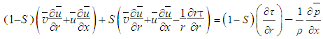
2. The New Mathematical Approach
- It is often possible to find two or more terms in an equation which dominate the solution, other terms giving only small corrections to the value obtained by neglecting them entirely. In neglecting the small terms, one must respect the Kruskal’s principle of maximal balance which states that no term should be neglected without a good reason [2]. In maximal balance, the comparable terms constitute a maximal set and the remaining small terms belong to a negligible set. The NMA described herein goes further and states that the negligible set, if it retains the essential physics of the original equation, may be called a minimal set which acts like an additional equation. Thus NMA may provide additional equations to get the closed system of equations from the unclosed one.
2.1. Algebraic Basis of NMA
- The mathematical justification for NMA is sought through an algebraic equation
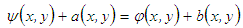 | (1) |
 | (2) |
 | (3) |
3. Applications of NMA
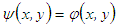
- NMA is applied to the unclosed governing equations for the two-dimensional (2D) turbulent boundary layer and round jet flows shown in Figs. 1 and 2. Boundary layers are wall shear flows where the fluid viscosity, no matter how small, enforces the no-slip condition at the solid wall. This viscous constraint gives rise to viscosity dominated characteristic velocity and length near the wall while turbulence dominated ones are found away from the wall. On the other hand, jets are free shear flows where fluid coming out from circular orifice mixes with the surrounding fluid and develops through three successive distinct regions, namely initial, intermediate and developed regions. Initial region is characterized by the presence of a potential core that is in laminar state, intermediate region by the transition state and developed (self-similar) region by the fully turbulent state. This jet grows non-linearly in the developing (initial and intermediate) regions and linearly in the developed region. The unclosed governing equations, additional equations due to NMA, primary closed form equations, secondary closed form equations, and their initial and boundary conditions are presented in this section.
 | Figure 1. Schematic of a plane boundary layer flow |
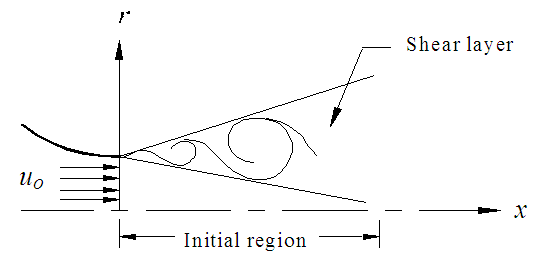 | Figure 2. Schematic of a round free jet |
3.1. Unclosed Governing Equations
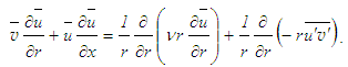
- Continuity and RANS equations governing the 2D axisymmetric turbulent flow
 for a constant property fluid in cylindrical co-ordinates
  are
are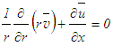 | (4) |
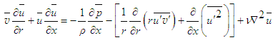
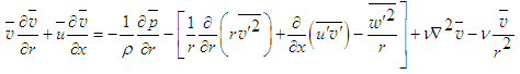 | (5) |
 | (6) |
 and
and  are the mean and fluctuating velocity components, similar are other quantities,
  and
and  are zero by the circumferential symmetry, ν is the fluid viscosity. The above continuity and RANS equations represent the governing equations for 2D plane turbulent flow
  in Cartesian co-ordinates (x, y, z) upon substitution of the free
 and
and  in them. The system of Eqs. (4)-(6) is not closed because there are more unknowns than the number of equations. In the next section, this unclosed set of equations is made closed by using the additional equation.
3.2. Additional Equation due to NMA
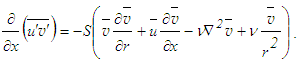
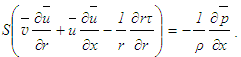
- Dimensional analysis provides a great deal of understanding of the physics involved in the governing equations of a phenomenon that is indispensable in determining both the maximal and minimal sets of the equations. In view of this, dimensional analysis of the RANS equations is carried out by considering the characteristic mean velocity U, velocity fluctuation u, flow width δ and flow length L as the scales of mean and turbulence velocities, diffusion and convection lengths, respectively, with the assumptions [10] that u is comparable to U and δ is comparable to L. Using these velocity and length scales, the orders of magnitude of the terms of Eq. (5) are estimated as follows:
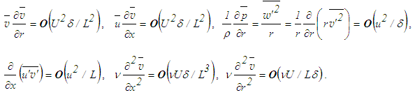 The terms of Eq. (5) are written in the order of their magnitudes as
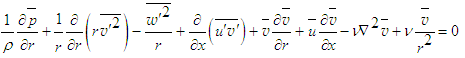 | (7) |
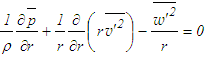 | (8) |
 | (9) |
 with the left side of this equation provides
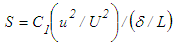 | (10) |
 and
and  and other scales remain the same. In case of free jet, only the scales u and δ change through the flow regions, marked by the difference in the flow state [6]. That is in some flow areas some terms are larger than others and relations between the terms vary in different flow areas. The scaling parameter which comprises of an arbitrary constant and some flow scales, accounts the variation of those relations through its transverse and axial dispersions.
3.3. Primary Closed Form Equations
- Equation (6) by the order of magnitude reasoning and uniform pressure assumption for thin shear flow (δ/L<<1) reduces to
 | (11) |
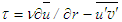
3.4. Secondary Closed Form Equations
- Comparison of unclosed equations in Sect. 3.1 with closed equations in Sect. 3.3 shows that
 and
and  are left unknown. With a view to obtain the equations for the unknown terms, Eq. (5) may be written as
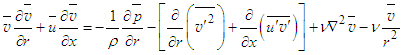 | (12) |
 and
and  are equal in axisymmetric flow and
  can be solved from this equation for the known
  . Afterwards
  can be calculated from Eq. (5) because all other quantities are already known.Neglecting the small viscous term, Eq. (6) may be read as follows
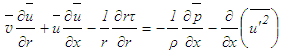 | (13) |
 is the effective shear stress. In order to solve the mean static pressure
  , Eq. (13) may be written by neglecting the small normal stress term as
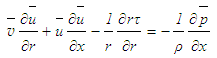 | (14) |
 | (15) |
 | (16) |
 is
is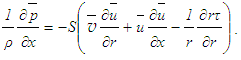 | (17) |
 may be obtained from Eq. (13) as
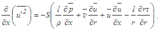 | (18) |
 can be solved by scaling Eq. (12) in the form
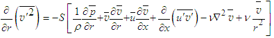 | (19) |
 can be solved by scaling Eq. (5) as
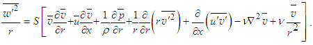 | (20) |
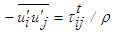
 does not appear in the RANS equations for plane boundary layer flow to add to the closure problem. So it can be obtained from the turbulent stress tensor
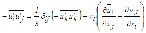 | (21) |
 and
and 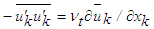 , and in 2D flow for i=j=3 reduces to
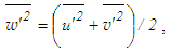 | (22) |
3.5. Initial and Boundary Conditions
- In boundary layer flow, the initial conditions are
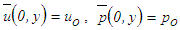 and
and  where uo and po are the uniform free-stream velocity and pressure, and
  is the general flow variable. The boundary conditions are
  attains free-stream values at the boundary layer edge,
  at the outflow and
  at the wall.In free jet flow, the initial conditions are
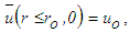
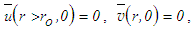
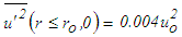 and
and 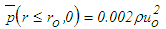 where ro and uo are the radius and uniform velocity at the jet exit. The boundary conditions are
  attains ambient conditions at the jet outer edge,
  at the outflow and
  at the axis of symmetry except
  .
.4. Numerical Methods
- It is already mentioned that eddy viscosity concept is the core of all turbulence closure models. As a result, hardly there is any standard numerical scheme for solving the closed form Eqs. (4), (9) and (11). This necessitates to writing the momentum equation (11) in the form
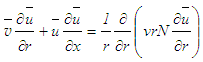 | (23) |
 and
and 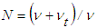 , and also necessitates to writing Eq. (9) as
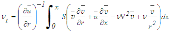 | (24) |
 is the eddy viscosity and N is the normalized effective viscosity.Further N is written in a recurrence relation, using the trapezoidal integration formula with the first degree polynomial and Eq. (24) in
 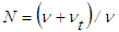 , in the form
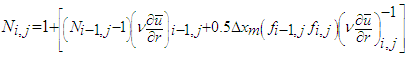 | (25) |
 and
and | (26) |
 and
and  . There second-order upwind interpolation is used for convective coefficients of Eq. (23). The solutions of
 and
and  are obtained from Eqs. (17)-(20) by writing them in finite difference form except Eq. (19) in the integral form for the solution of
  . In boundary layer flow, the solution of
  is obtained by using Eq. (22).
4.1. Grid Specifications
- Schematic of the computational domains for the boundary layer is Lx=0.4m and Ly=0.6m in x- and y-directions as seen in Fig. 1 and for the jet flow Lr=10d and Lx=30d in r and x- directions where d=0.04m is the jet diameter at the exit as in Fig. 2. Grid spacing is uniform in x- and variable in y- directions such that yj+1=Kyj and Δy1=Ly(K-1)/(Knj-1) where K =1.12 for the boundary layer and K =1.02 for the jet flow. Here all the flow properties are located at the same grid point as the pressure gradient is absent in the set of primary closed form equations to be solved. The under-relaxation factors used for
 and N are equal to 0.7 for each. The used numerical scheme is second order accurate and found to provide converged solution in 19 iterations which is accurate to six decimal places for the mean velocity
  . To avoid the necessity of special grid specifications near the wall to account the steep variation of flow properties, certain variation of
  is assumed within y/δ<0.05 in accordance with Townsend [13] and Klebanoff [14] data, instead of
  in Eq. (24), where κ =0.4 is the von Karman constant and
  is the friction velocity.
4.2. Grid Convergence Test
- Grid convergence test is carried out with the three different grid sizes termed as coarse, medium and fine for nixnj equal to 431x61, 461x66 and 501x71 where ni and nj are the number of grid points in x and y-directions for the boundary layer flow, and 1021x121, 1111x134 and 1201x145 in x and r-directions for the jet flow. Figure 3 shows the transverse profiles
 of the boundary layer at x/L=0.5 for the three different grid resolutions with Re=8x10⁵ where Re=uoL/ν is the Reynolds number. Figure 4 exhibits the radial profiles
  of the round jet with Re=3104 at the location of x/d=3 for the three different grid resolutions where Re=uod/ν. Grid refinement shows successful convergence with the three grid sizes. The results presented in this paper are obtained by using the fine mesh.
 | Figure 3. Mean velocity profiles at x/L=0.5. Grid points  |
 | Figure 4. Mean velocity profiles at x/d=3. Grid points  |
5. Results and Discussion
- The unclosed set of equations governing the turbulent flow, continuity and RANS, is made closed using the additional equations due to NMA. The closed set of Eqs. (4), (23) and (25) is solved both for the boundary layer and free jet flows for the given initial and boundary conditions using FINS and TDMA. Details of the scale factor S for calculating
 and
and  from Eq. (9) and Eqs. (17)-(20), respectively, are described in the next subsections. The flow development, mean velocity, turbulent shear and normal stresses, and mean static pressure from the present simulation for both types of flow are presented in this section, and compared with the experimental data of Klebanoff [14] for Rθ=7500, Murlis et al. [15] for Rθ=5000, Coles [16] for Rθ=5000 and McQuaid [17] with little air injection
  for Rθ=5000 for the boundary layer flow, and compared with the experimental data of Fellouah et al. [18] for Re=3104, Fellouah and Pollard [19] for Re=3104 and Hussein et al. [20] in the self-similar region (x/d ≥ 30) for Re=9.6104 for the jet flow.
5.1. Boundary Layer Flow
- Simulation is made for the turbulent boundary layer due to air flow over the flat plate with zero pressure gradient at Rθ=2170 (Re=8x10⁵) where Rθ=uoθ/ν is the Reynolds number and θ is the momentum thickness. The shapes of
 and
and  are identical [21] to
  that renders Eq. (10) to S=C1. The numerical scheme is found to converge to a stable solution for C1=3.2 which appears in Eq. (25) through
  .
.5.1.1. Flow Development
- Development of the boundary layer is shown schematically in Fig. 1 where its thickness δ is located at
 . The growths of δ and θ represented by the Reynolds numbers Rδ and Rθ are shown in Fig. 5 against x/L where Rδ =uoδ/ν. There the staircase boundary layer edge obtained from the present simulation is shown by the best fit. It seems from the figure that boundary layer thickness is one order higher than momentum thickness which is consistent with the theoretical results [21].
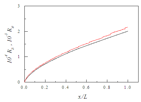 | Figure 5. Streamwise growth of the boundary layer.  |
 against Rθ where
  is the wall shear stress. Muralis et al. [15] data of friction coefficient added in the figure for comparison are seen in acceptable agreement with that of the present simulation. Figure 6(b) shows the streamwise variation of the shape factor H against Rθ where H is the ratio of displacement thickness to momentum thickness with their usual definitions. The value of H in the figure indicates a turbulent flow although the Reynolds number is low. Comparison shows that Coles [16] data are in good agreement with that of the present simulation.
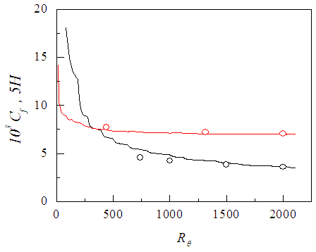 | Figure 6. Streamwise variation of (a) friction coefficient: present  , Muralis et al. data [15] (o), (b) shape factor: present , Muralis et al. data [15] (o), (b) shape factor: present  , Coles data [16] , Coles data [16]  |
 for the boundary layer is plotted in Fig. 7 against the transverse distance y/L at the streamwise locations x/L=0.3, 0.6 and 1.0. As the streamwise distance increases, the boundary layer grows and velocity within it decreases due to increasing loss of momentum at the wall. Dimensionless mean velocity
  is shown against
  in Fig. 8 at three different locations x/L=0.3, 0.6 and 1.0. Mean velocity profiles follow the log-law
 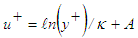 , with constants κ=0.4 and A=5 which are close to their widely known values. The velocity profiles have the logarithmic region between
  and
and  where the upper limit depends on the Reynolds number of the flow.
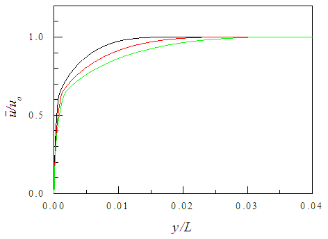 | Figure 7. Mean streamwise velocity profiles at 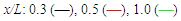 |
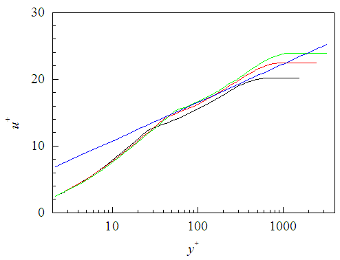 | Figure 8. Mean velocity profiles in semi-log axes. Lines as in Fig. 7. Log-law  |
5.1.2. Flow Properties
- Mean streamwise velocity
 is plotted in similarity co-ordinates in Fig. 9 at x/L=0.3, 0.6 and 1.0 using the velocity scale uo and length scale δ. The scalings are found to collapse the velocity profiles very well. The
  velocity profile of the present results is compared with Klebanoff [14] data and found to be in good agreement. Mean transverse velocity
  is plotted in the similarity co-ordinates
 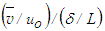 and y/δ in Fig. 10 which shows good collapse of the transverse velocity profiles right from the wall outward. In the figure, these velocity profiles show an outward flow at all x- locations of the boundary layer. It is noteworthy that the plot of
  -velocity profiles does not collapse in similarity co-ordinates
  and y/δ (not shown) which is consistent with the existing literature [22].
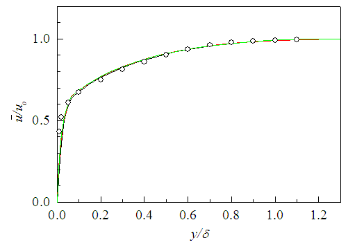 | Figure 9. Mean streamwise velocity profiles. Lines as Fig. 7. Klebanoff data [14] (o) |
 | Figure 10. Mean transverse velocity profiles. Lines as Fig. 7 |
 profiles in similarity co-ordinates
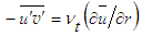
  and y/δ right from the wall at the positions x/L=0.3, 0.6 and 1.0. This shear stress is calculated using the eddy viscosity formula
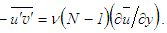 | (27) |
 | Figure 11. Reynolds shear stress profiles at 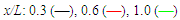 . Klebanoff data [14] (o) . Klebanoff data [14] (o) |
 | (28) |
 | Figure 12. Reynolds shear stress by Eq. (9). Lines and symbol as in Fig. 11 |
 is obtained from Eq. (17). The normalized pressure
  is plotted in Fig. 13 against y/δ at the streamwise positions x/L=0.3, 0.6 and 1.0. The obtained solution requires
  close to the wall and
  away from the wall. The profile of
  at x/L=1 (Rθ=2170) is compared with the experimental data [17] at Rθ=2060 and found in qualitative agreement where the disagreement is due to lower
  in the experiment induced by the fluid injection.
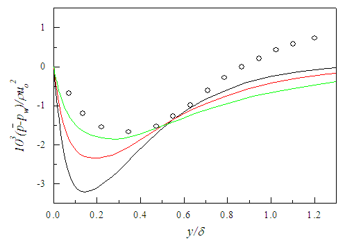 | Figure 13. Mean static pressure profiles. Lines as in Fig. 11. McQuaid data [17] (o) |
 and
and  are obtained from Eqs. (18) and (19), respectively, for S =0.025 and S =1.3. The solution of
  is obtained using Eq. (22). Figure 14 displays the stresses
  and
and  as functions of y/δ at x/L=1. Klebanoff [14] data for the normal stresses added for comparison exhibit good agreement with that of the present simulation.
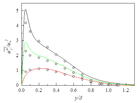 | Figure 14. Turbulent stress profiles at  . Klebanoff data [14] (o) . Klebanoff data [14] (o) |
5.1.3. Estimation of Scale Factor
- Scale factor S is estimated for calculating
 from Eq. (9),
  and
and  from Eqs. (17)-(19) by comparing the orders of magnitude of the shear stress term with the inertia as S=C1, comparing the pressure with the shear stress as S=C2(δ/L), comparing the axial normal stress with the pressure as S=C3 and comparing the transverse normal stress with the pressure as S=C4, respectively, where C1, C2, C3 and C4 are constants. Equation (17) for
  possesses parametric scale factor while Eqs. (18) and (19) for
  and
and  possess constant scale factor. As a result, the solution of
  requires a small value of C2 near the wall and a large value away from the wall due to the presence of viscosity dominated flow scales near the wall and turbulence dominated one away from the wall.
5.2. Round Jet Flow
- Simulation is made for the round free air jet with 40 mm diameter and top-hat velocity at the exit with Re=3104. The numerical scheme is found to converge to produce a stable solution for
 at x/d ≤15 and for S=1 at x/d >15 where S appears in Eq. (25) through
  . Such expressions for S come from the reduction of Eq. (10) at x/d ≤15 due to u2/U2 ~x and δ/L~x-0.5, and at x/d >15 due to the constant values of both u2/U2 and δ/L.
5.2.1. Flow Development
- In the present simulation, initial region terminates at x/d=5.2 at which uc=0.98uo and intermediate region terminates at x/d≈15 beyond which the jet grows linearly. The obtained location for the latter region is close to the data of Ferdman et al. [23] for Re=2.4104 and Xu and Antonia [24] for Re=8.6104. Direct numerical simulation of a round jet performed by Boersma et al. [25] for Re=2.4103 shows that self-similar state of the Reynolds stress appears at 20<x/d<35, although general consensus [26] is that fully developed region occurs approximately at x/d≥30. The conditions for self-similarity obtained from axial RANS equation (11) by neglecting the viscous effect dictate U=U(x) or constant [27] but presence of the pressure or normal stress gradient in the equation restricts U to be constant.Axial decay of the centerline mean velocity uc is shown in Fig. 15 that follows the inverse relation with downstream distance given by
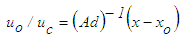 | (29) |
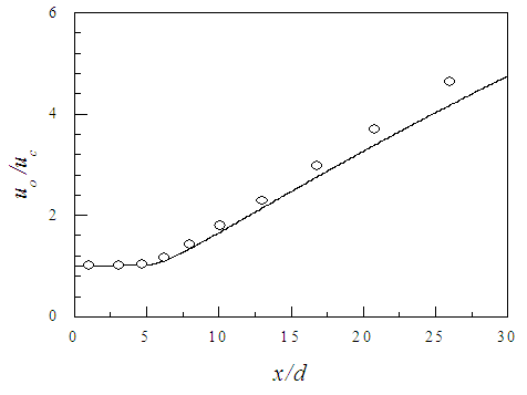 | Figure 15. Centerline mean velocity. Present  , Fellouah et al. data [18] (o) , Fellouah et al. data [18] (o) |
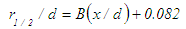 | (30) |
 | Figure 16. Growth of jet half-width. Present  , Fellouah and Pollard data [19] (o) , Fellouah and Pollard data [19] (o) |
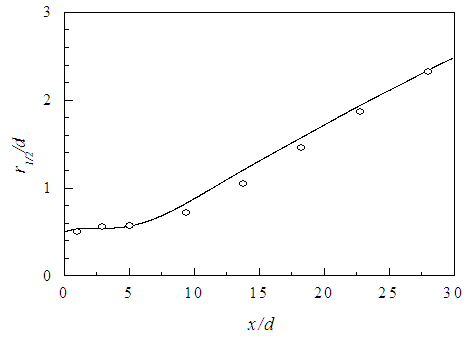
 is presented in Fig. 17 against the radial distance r/d at the axial locations x/d=3, 10 and 15. As the axial distance increases, the jet grows due to entrainment of the ambient fluid and its maximum velocity decreases due to the loss of momentum by the interaction with the ambient fluid.
 | Figure 17. Mean axial velocity profiles at 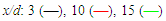 |
5.2.2. Flow Properties
- Radial profiles of mean axial velocity
 are plotted in Fig. 18 at axial positions x/d=3, 10 and 15. Fellouah et al. [18] data added for comparison show reasonable agreement with those of the present simulation. Again, radial profiles of this velocity are displayed in Fig. 19 in similarity co-ordinates
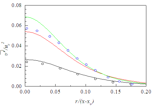
  and r/(x-xo) at x/d=10, 20 and 30, and found in good collapse. Hussein et al. [20] data of -velocity are found in acceptable agreement with the present results. Mean radial velocity
  is plotted in Fig. 20 in similarity axes
  and r/(x-xo) at x/d=10, 20 and 30. The
  -velocity in Pope [10] from Hussein et al. laser doppler anemometer data included for comparison are found in reasonable agreement with that of the present simulation but run off at r/(x- xo)>0.15 and the velocity becomes negative. This is because of more decay of the jet in Hussein et al. (A-1=0.17) causes more entrainment of the ambient fluid towards the jet centerline compared to the present simulation (A-1=0.16).
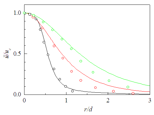 | Figure 18. Mean axial velocity profiles. Lines as in Fig. 17. Fellouah et al. data [18]  |
 | Figure 19. Mean axial velocity profiles at 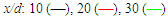 . Hussein et al. data [20] . Hussein et al. data [20]  |
 | Figure 20. Mean radial velocity profiles. Lines as in Fig. 19. Data from Pope [10]  |
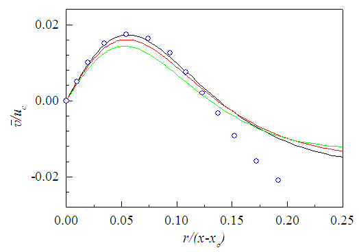
 is depicted in Fig. 21 against r/d at x/d=3, 10 and 15. This shear stress is calculated using eddy formula in Eq. (27). The profiles of
  are seen in satisfactory agreement with Fellouah et al. [18] data, although the stress level is somewhat different in the simulation. Lower decay of the jet in the present simulation (A-1=0.16) than the experiment (A-1=0.18) causes lower level of
  as appears in the figure for
  at x/d=3 but normalization by
  masks this fact at x/d=10 and 15. This shear stress is plotted again in Fig. 22 against r/(x-xo) at x/d=10-30. Data of Fellouah et al. [18] and Hussein et al. [20] added for comparison show close agreement with that of the present simulation.
 | Figure 21. Reynolds shear stress profiles at  . Fellouah et al. [18] . Fellouah et al. [18] 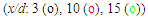 |
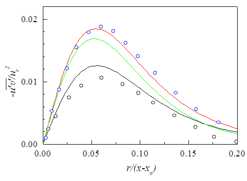 | Figure 22. Reynolds shear stress profiles at x/d:  . Fellouah et al. [18] (o), Hussein et al. [20] . Fellouah et al. [18] (o), Hussein et al. [20]  |
 is calculated from Eq. (9) for S=0.043 in the initial region,
  in the intermediate region and
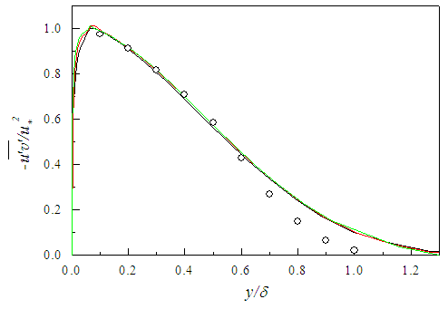
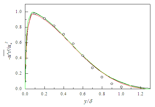
  in the developed region where S for different regions are obtained by simple comparison of magnitudes of the appropriate terms as shown in the next section. This calculated shear stress is seen to increase rapidly in the downstream from x/d=10-30 as shown in Fig. 23 indicating that S cannot accommodate the axial evolution of turbulent shear stress unlike the boundary layer flow. This is because turbulent stresses gradually increase and then decrease along the jet flow, i.e. their slopes change from positive to negative contrary to the boundary layer flows as observed in experiments and simulations (e.g. [29, 30]). While
  obtained by comparing the magnitudes of the terms as above but with −S instead of +S at x/d>15 (exemplified later) to account such negative slope effect (NSE) proves to be able to predict the evolution of the shear stress as demonstrated in Fig. 24. Fellouah et al. [18] and Hussein et al. [20] data added for comparison are found in good agreement with the present simulation.
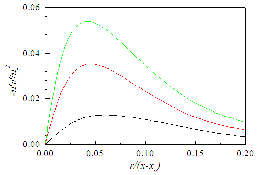 | Figure 23. Reynolds shear stress by Eq. (9) without NSE. Lines as in Fig. 22 |
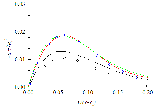 | Figure 24. Reynolds shear stress profiles by Eq. (9) with NSE. Lines as in Fig. 22. Data of Fellouah et al. [18] (x/d: 10 (o)) and Hussein et al. [20]  |
 is shown in Fig. 25 against r/d at the axial positions x/d=3, 10 and 15. The solutions are obtained for
 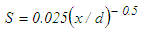 in the initial region,
 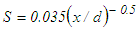 in the intermediate region and
 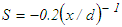 in the developed region. Here S for the developed region of the jet is obtained by taking NSE because pressure also changes slope at some distance downstream along the flow. Figure 26 displays
  as a function of r/(x-xo) at x/d=10-30 where the centerline pressure is seen to decrease in the downstream as may be observed from Quinn [29] data.
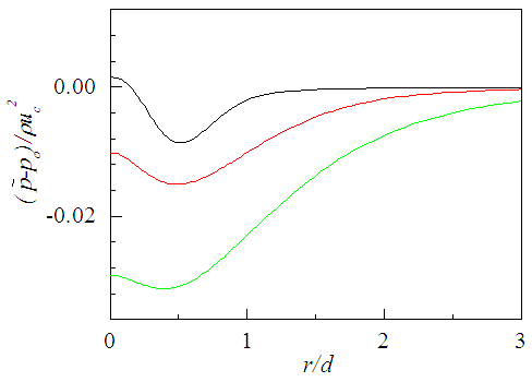 | Figure 25. Mean static pressure profiles at 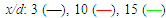 |
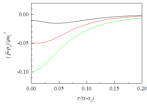 | Figure 26. Mean static pressure profiles at 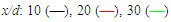 |
 is obtained from Eq. (18) along with the continuity equation for the scale factors
 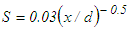 for the initial region,
 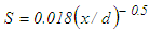 for the intermediate region and S=-0.06 for the developed region considering NSE by equating the orders of magnitude of the proper terms. The normalized stress
  is plotted in Fig. 27 against r/d at x/d=3, 10 and 15. Fellouah et al. [18] data of the normal stress provided for comparison are found in excellent agreement with those of the present simulation. Obtained solution with NSE at x/d>15 proves to be able to predict the axial evolution of the normal stress as observed in Fig. 28. While calculated normal stress without NSE, like the shear stress, are seen to increase rapidly in the downstream from x/d=10-30 (not shown). Fellouah et al. [18] and Hussein et al. [20] data included there for comparison are found in reasonable agreement with the present simulation.
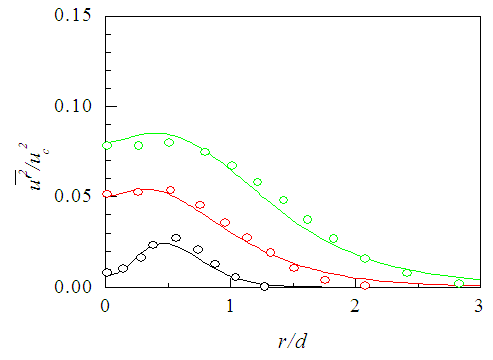 | Figure 27. Axial normal stress profiles. Lines as in Fig. 25. Fellouah et al. data [18] 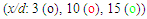 |
 | Figure 28. Axial normal stress profiles with NSE. Lines as in Fig. 26. Data of Fellouah et al. [18] (x/d: 10 (o)) and Hussein et al. [20]  |
 is obtained by integrating Eq. (19) along with the continuity equation for
 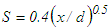 in the initial region, S=0.075 in the intermediate region and S=0.056 in the developed region. The scale factors are determined by comparison of the magnitudes of the suitable terms of the equation where
  does not appear as axial derivative and does not require to consider NSE for the developed region. The stress
  is presented in Fig. 29 against r/d at x/d=3, 10 and 15. Fellouah et al. [18] data of
  (taken here about twice of their
  being the values are somewhat less than the expected) added for comparison are found in excellent agreement with those of the present simulation. Figure 30 displays
  against r/(x-xo) at x/d=10-30. Fellouah et al. [18] and Hussein et al. [20] data included for comparison show fair agreement with that of the present simulation.
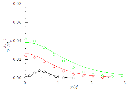 | Figure 29. Radial normal stress profiles at  . Fellouah et al. [18] . Fellouah et al. [18]  |
 | Figure 30. Radial normal stress profiles at 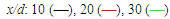 . Data of Fellouah et al. [18] (x/d: 10(o)) and Hussein et al. [20] . Data of Fellouah et al. [18] (x/d: 10(o)) and Hussein et al. [20]  |
 is obtained from Eq. (20) along with the continuity equation for S=0.012 at x/d ≤30. The stress
  is depicted in Fig. 31 against r/d at x/d=3, 10 and 15. The profiles of
  are displayed in Fig. 32 against r/(x-xo) at x/d=10-30 where Hussein et al. [20] data added for comparison are found in acceptable agreement.
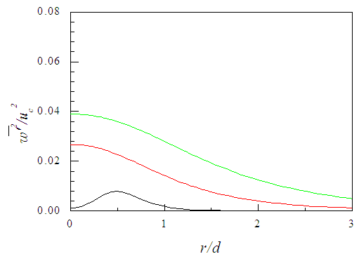 | Figure 31. Azimuthal normal stress profiles. Lines as Fig. 29 |
 | Figure 32. Azimuthal normal stress profiles. Lines as Fig. 30. Hussein et al. data [20]  |
5.2.3. Estimation of Scale Factor
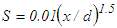
- In order to estimate the scale factor, nonlinear growth of the jet in the developing region (x/d≤15) is assumed as
 and linear growth in the self-similar region (x/d>15) as
  in accordance with the literature [24, 31]. The assumption of linear growth of the jet at x/d>15 is in excellent agreement with that of the present simulation. Experimental and computational data (e.g. [29, 32]) show that
  increases rapidly as linear in x at x/d ≤15 and then decreases as x-1 at x/d>15 indicating the axial variation of the fluctuating velocity scale u for the same regions. In determining S for Eq. (9), equating of the orders of magnitude of
  and
and  for the viscosity dominated initial region (x/d≤5) yields S=C1, and equating of
  and
and  for 5≤x/d≤15 yields S=C1x1.5. Then comparison of the magnitudes of
  and
and  along with NSE for x/d>15 provides
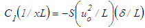 | (31) |
 and
and  from Eqs. (17)-(20), respectively, by the comparison of magnitudes of the appropriate terms. In estimating S for Eq. (17), comparison of the pressure and shear stress for x/d ≤15 provides S=C2/x0.5 with two different values of C2 for the initial and intermediate regions and equating of the pressure and inertia along with NSE provides S=-C2/x for x/d>15. In evaluating S for Eq. (18), comparison of the normal stress and shear stress for x/d ≤15 provides S=C3/x0.5 with two different values of C3 for the initial and intermediate regions and equating of the normal stress and pressure for x/d>15 along with NSE yields S=-C3. Evaluation of S for Eq. (19) is made by simply equating the radial normal stress and shear stress as S=C4 x0.5 for the initial region and equating the normal stress and pressure yields S=C4 with two different values of C4 for the intermediate and developed regions. S is evaluated for Eq. (20) by equating the azimuthal and radial normal stresses as S=C5 with a single value because axisymmetry requires that
  over the entire jet flow.
6. Further Discussion
- Computational results show that C1= 3.2 for the additional Eq. (9) in the boundary layer flow implying that
 and
and  are of equal orders of magnitude but
  while C1=1 at x/d>15 for the jet flow implying that
  and
and  are of equal magnitudes. Moreover,
  is seen larger than
  in the initial region of the jet at the time of calculating the shear stress from Eq. (9). In most turbulent shear flows, Reynolds normal stresses bear the relation
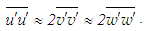 | (32) |
 after Bradshaw et al. [33] and the shear correlation coefficient
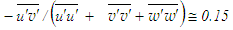
 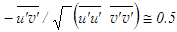 after Klebanoff [14] along with Eqs. (8) and (32), the conditions
  can be derived for the boundary layer flow. In the free shear flow, the values of 0.135 and 0.4 for the turbulent structure parameter and the shear correlation coefficient after Pope [10] give the conditions
  . Results from the present simulations at the last axial position of their calculation domains are seen to closely satisfy the above conditions across some fraction of the shear layer for both types of flow. It is to be noted for the boundary layer flow that in addition to the agreement with Klebanoff [14] data, the estimate of
  using Eq. (22) are found in excellent agreement by DeGraaff and Eaton [30] with their experimental data.
7. Conclusions
- Two-dimensional continuity and RANS equations for the mean motion occur with six unknowns for the boundary layer flow and with seven unknowns for the jet flow. In this study, one additional equation for the boundary layer flow while two additional equations for the jet flow are obtained from the transverse RANS equation using NMA and two other equations are obtained from the streamwise RANS equation using extended NMA to achieve the turbulence closure. The closed form equations are solved numerically that provide solutions for the mean streamwise velocity, mean transverse velocity, mean static pressure, and Reynolds shear stress and normal stresses. Results extracted from the simulation of both types of flow are found in overall agreement with the existing experimental data that proves the effectiveness of NMA in achieving the complete turbulence closure.