1. Introduction

One of the problems related to computational methods is capturing the region with sharp gradients (sudden changes). This state occurs in flow when we encounter suddenly changes in flow variables. These kinds of changes are known as discontinuities. First-order approximation methods captured the sharp discontinuities with high error, while high-order shock-capturing methods are associated with non-physical fluctuations. For this purpose, the high-order methods without fluctuation (High Resolution Schemes) are designed in such a way to prevent the fluctuations, as much as possible, by having acceptable accuracy. The classical computational methods such as Jameson, TVD and ENO used in aerodynamic applications for computing compressible flows with shock waves are of these kinds. Since the basis of these methods is based on increasing the numerical dissipation in sudden and rapid changes in flow variables, so a relative decline will be observed in the accuracy said that the most important part of the finite volume method is calculating the passing flux through the cell of these regions. Considering that different characteristics have different dissipation from each other. The main important part of the finite volume method is calculation of the flux in the cell walls. Researchers have introduced a lot of methods for calculating these fluxes in a more accurate and low-cost way. Godunov (1959) [1] for the first time used Riemann problem in the calculation of flux. Riemann problem is considered as a shock tube with two different pressure (two different speeds) that is separated by a diaphragm. Godunov solved Riemann problem for each cell walls. In fact, Godunov method needs the answer of the Riemann problem, and in a practical calculation, this problem is resolved millions of times. The problem of Godunov method is the direct use of the Riemann problem with its complete solution that when the problem is resolved million times, the computing time greatly increases. Because of this reason, Roe (1981) [2] used the approximation method for solving the Riemann problem. Roe method is based on Godunov method. For this purpose, Roe used method of linear averaging, and this method is known as the Roe averaging method. After Roe, other people reform his method and different plans had been proposed based on Roe method. Jameson (1981) [3] used averaging and artificial viscosity method for calculating the flux. In this method, Jameson used modified Rung-kutta fourth order to discrete the time. The greatest advantage of this method in addition to simplicity and its use in complex geometries is its high resolution in capturing shock in transonic flows. The work of Jameson.et al was a combination of numerical dissipation of second and fourth order based on flow gradients that, with two adjustable parameters, was considered for central difference. Although considerable improvement was obtained in the results, but setting two parameters to extract acceptable results in discontinuities must be found by trial and error for each problem. In other words, the choice of optimal dissipation term depends on the experience of working with code. In addition, the direction of waves motion in the hyperbolic flow was overlooked. Harten [4] introduced total variation diminution (TVD) in 1984. In this method, having a reduction trait in total variations of conservation laws for both hyperbolic scalar equation and hyperbolic equations with constant coefficients were the main goals. One problem of TVD methods was that it changed to the first order methods in the discontinuities, therefore, smooth variations of solutions was created in the shock wave and other discontinuities. Note that, in the first order methods in which the second and higher derivatives of Taylor expansion are overlooked, diffusion errors were created and consequently the solution dispersed to the surrounding points. Another method that was proposed by Harten (1977, 1978) [5-6] for flows with discontinuities was the combination of a first order scheme with an ACM (Artificial Compression Method) switch. In this method, ACM switch is operated as an artificial compression that appears in intensive gradients. Turkel et al (1987, 1997) [7] imposed a method called preconditioning to the density based algorithm, and showed that the usage of the new approach gave an aacceptable and accurate results of incompressible and small Mach numbers flows for solving compressible flow equations. Also in a recent study carried out by Razavi and Zamzamian (2008) [8], a new method based on density based algorithm and method of characteristics was presented by applying artificial compressibility method in order to solve incompressible fluid flow equations. Rossow (2003) [9] supposed a method to synthesize the density based and pressure based algorithms, which allows pressure based algorithm changes to the density based one. In this study, Riemann solver was studied in the incompressible flow regime, and solution algorithm is based on the pressure one. Synthesizing of this algorithm and density algorithm provides transition from incompressible to the incompressible flow regime, and it’s possible to solve both flows. Colella and Woodward [10] implemented the idea of using both first-order flux and anti-diffusion term as a limiting flux. In this procedure, the calculated optimal anti-diffusion is added to the first order flux. Montagne et al (1987) [11] compared high resolution schemes for real gases. This comparison showed that approximated Riemann solvers were reliable for real gases. One of the main researches based on TVD idea was the Duru and Tenaud works [12]. In the Mulder and Vanleer(1985) [13] and Lin and Chieng (1991) [14] showed that the best variable in view of the numerical solution accuracy was the kind of variable by using the limitations on initial variables ‘conservative and characteristic which were experimented in the unsteady one-dimensional flow. Yee et al (1985) [15] developed first order ACM of Harten to TVD method with different approach. Thereby, instead of reducing degree in capturing shock waves، order of accuracy remained at an acceptable level and demonstrated relative favorable capturing of high gradients (Shock). In another research، Yee et al (1999) [16] directly imposed ACM switch to the numerical distribution term (filter) of TVD method. In this work, basic scheme namely the central difference term in the flux approximation at the cell surface was in order of two, four, and six. Also ACM terms were appeared in discontinuity locations. Thus, in that zones of flow without any discontinuity‘Central Difference approximation was high and in exposing to the sudden changes in flow،numerical diffusion, which is less than the value of diffusion numerical second order TVD, are add to the Central difference term. Hatten (1983) [17] accomplished different designed in order to calculate and limit total amount of oscillation of variables or their error due to the idea of the total change (TVD).

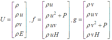
2. Governing Equations

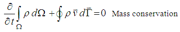
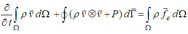
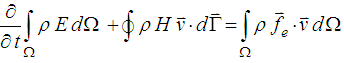
In this section, the mathematical formulating of the governing equations on compressible non-viscous flow used in all flow regimes and is known as Euler Equations, will be discussed. Euler equations for transiting flow from Ω volume and limited to Γ surface in the integral mode could be written as. Eqs.(1),(2),(3).

(1)

Momentum conservation:

(2)

Energy conservation:

(3)

That in the above equations, ρ is density, is the velocity vector, is the pressure, is external forces, E is internal

Energy and H is the enthalpy of the fluid that can be written as .Eq.(4).

(4)

The total internal energy of is defined as 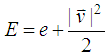and in this equation e is defined as and is the specific heat at constant volume. The above equations could be defined in a whole and compressive way. So that if U represents a vector or tensor of conservation variables, represents conservation vector fluxes and is a unit matrix, then it can be written as. Eq.(5).

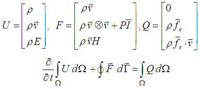(5)

If we write the above equation differentially and in vector mode, then we have .Eq.(6) as following:

(6)

In two-dimensional and unsteady flow, the Cartesian components of U vector and also F vector are defined by the following relations as .Eq.(7).

(7)

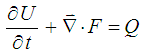
Where u and v are the components of velocity vector. In this case, equation (6) could be written in the Cartesian coordinate system as .Eq.(8).

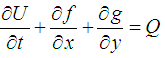(8)

The above equation is known as the Euler equation.

3. Calculation of Flux in an Oblique Surface

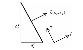
According to the practical problems, the computational grids are not always orthogonal, and grid lines are not along the flow; thus, the passing flux from the surface of cell could have component in both directions of x and y for each local direction; thus, changes must be created in the form of equations and the way of flux calculation to allow the calculations to be performed in non-orthogonal grids as well. In the most of researches conducted by Harten and Yee and other researchers, the method used frequently was finite difference, and computation was carried out in the computational grid which is different from physical grid; therefore, the matrix of left and right vectors and other flux parameters in the directions of Cartesian x and y have been used separately and unchanged. Finally, after calculations, conversion from local coordinates to the original coordinates would apply to them, but because at the present work the grid and discretization of governing equations are based on finite volume and computational grid is the physical grid itself, the considered method to calculate flux is based on the method of Hirsch(1990), and it is in the form that all flux sentences and its components at local directions of are decomposed to y and x components and added together. For this task, it is necessary to investigate the grid geometry and the position of the cell surface to the adjacent cells centers. Geometry used in calculating the flux is shown in fig.1.

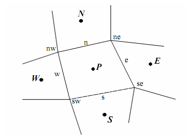Figure 1. Geometry used in calculating the flux

3.1. Calculation of Flux at e Surface

In order to calculate the passing flux in the e surface of cell, the surface shown in the figure 1 is considered. If this surface is separately to be investigated, an arbitrary position of that surface in the locational coordinate (ξ,η) is related to the main coordinate (x,y) as figure 2.

Figure 2. Cell surface e in the local coordinates

The geometric relations for the above state could be written as .Eq.(9).

(9)

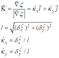
So, according to the symbols of figure 1, can be written as equation (10):

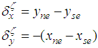(10)

As it can be seen, and are the Cartesian components of unit vector of . This unit vector is perpendicular to the surface of cell, and put along the locational direction. Noticing to the above equations, flux of velocity vector in direction can be defined as Eq.(11).

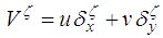(11)

Conservative vector of variables is shown by , and conservative vectors of mass flux, momentum and energy in each of adjacent cell center of e surface are as. Eq.(12).

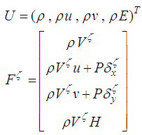(12)

Flux for each desired cell in e surface could be calculated as. Eq.(13).

(13)

In above equation, in hyperbolic equation system, for the two-dimensional flow four eigenvalues in above surface are as. Eq.(14).

(14)

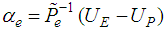
sign means that matrix is defined at the surface of e cell, and all of its elements are based on Roe averaging method.

And also, the characteristic variable α in e surface from multiplying each row of the matrix of left special vector of in conservative variables could be calculated as. Eq.(15).

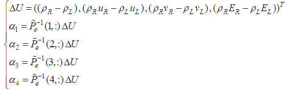(15)

The above equations, in general and as a vector, could be written as. Eq.(16).

(16)

In these equations, subscript relations of are related to the center of left e cell and the center of right e cell surface, respectively. And also represents the row i of the left eigenvectors matrix. And in the relation (13) is the column i of matrix, as .Eq.(17).

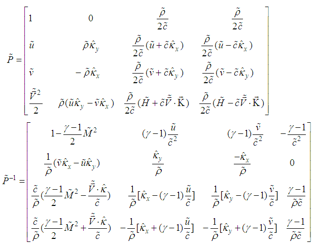(17)

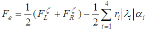
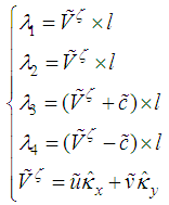
Yee (1986) and Yee et al. (1999) proposed the following equation for diffusion sentence based on TVD approximation of (2^nd order –upwind TVD) the second order upstream method for local discretization as .Eq.(18).

(18)

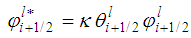
Function has been suggested as .Eq.(19).

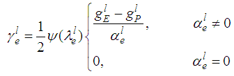(19)

In the above equations, is eigenvalue related to lth characteristic in the surface of e cell and is the limiting function related to lth characteristic in the center of the ith cell, and is characteristic variable in surface of e cell that is equal to column l of matrix , and finally, function is entropy function. Harten and Hyman (1983) suggested the above condition as .Eq.(20).

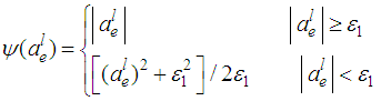(20)

That in this equation is zero for problems with moving shock waves is usually and is considered as a small amount for stationary waves. Different functions could be selected for limiter function of in the center of cell. Yee at al. (1999) proposed a number of these functions, and one of these functions is used in the present study which is as .Eq.(21).

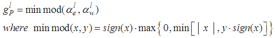(21)

Also, to avoid any problems in the implementation of the computer program, Yee et al (1999) introduced the following relations for the entropy and Gama functions as. Eq.(22).

(22)

Which in the all of computations was considered equal to , and was considered equal to 0.0625.

4. Reduction of TVD Error Using Artificial Compression Method (ACM)

As it was explained, when discontinuities is occurred, high resolution method such as TVD and ENO prevent to create oscillations by decrement of order while the diffusion is increased. Hereby, the accuracy of shock waves capturing is decreased in the discontinuities; therefore, finding a method for modifying this phenomenon is essential. Harten introduced a new method for increasing the accuracy of first order scheme in the shock wave capturing of discontinuities zones. Yee et al. used above method for viscous flow as. Eq.(23).

(23)

In this equation, the diffusion function is combined by TVD and anti-diffusion functions (Harten switch) in which the anti-diffusion function is directly imposed to it.

(24)

(25)

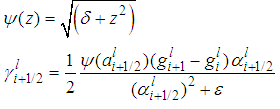
In this equation, is the anti-diffusion function at the surface of i^th cell related to the l characteristic and k is a variable that depends on the properties of problem. In this study, in order to increase the accuracy and decrement of diffusion in discontinuities, another approach is considered for imposing the ACM to diffusion term of TVD. With noticing to the previous points, ACM cannot be imposed to diffusion term directly, therefore, the anti-diffusion function is imposed to the limited function, which is put into the diffusion term and affects on it. The used method is as. Eq.(26).

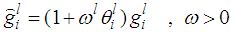(26)

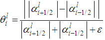
As it can be seen, the g function is replaced by the generated limited function in the diffusion term of TVD. is the coefficient of ACM in this equation. Because each wave (linear and nonlinear wave) has a particular diffusion, we have different coefficients relative to the other characteristics for each characteristic. is defined as equation 27 in i^th cell for each characteristic of l.

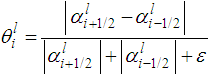(27)

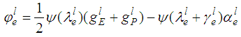
α is the characteristic variable computed at the surface of cell. is a coefficient that is different for various characteristics and is function of flow physics. Thus, it’s calculated by try-error method for a specific flow. Based on the mentioned equations, the new limited function is greater than the limited function of TVD method. As a result, accuracy and convergence of solution are improved, which affect on improvement of the shock wave capturing. But, with increment of and consequently the limited function, the diffusion is too decreased and the convergence procedure is probably interrupted. Thus, should be defined in a specific range or should be have an optimum value for a specified flow, which in that values, increment of the accuracy doesn’t happen with more convergence reduction and computation time increment, which is discussed in the next section.

5. Results and Discussion

This section discusses about the outlet results from the solution of inviscid flows by TVD, and ACM methods and compares them together. It’s also explained about the effect of numerical diffusion reduction on the results. The present topic is unsteady flow in sonic pipe which results compared with analytical solution and is a suitable experiment in the computational fluid dynamic (CFD) for compressible flows computations.

5.1. Unsteady Flow in Sonic Pipe

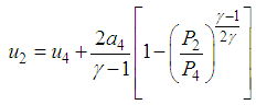
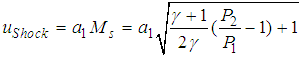
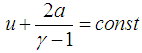
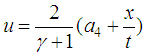
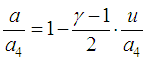
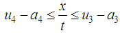
Since the flow in the sonic pipe includes three types of discontinuities and also the analytical solution of flow is possible, thus it is one of the study cases for the numerical methods. Using the initial values governing to the pipe and according to Fig3, by using perfect gas equations, analytical solution of the flow in the desired times can be done. The result is an implicit equation solved by an iterative method. Final equations for the P₄>P₁ are as. Eqs.(28),(29),(30) and (31).

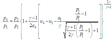(28)

(30)

(31)

a₁ is sound speed in zone 1, a₄ is the sound speed in the zone 4, R is gas constant, C_v, C_p and γ, are specific heat at constant volume, specific heat at constant pressure and the specific heat ratio respectively. By solving eq28 with initial values P₁ and P₄, P₂ is obtained. Given P2, the other variables can be calculated from the following equations (32) and (33).

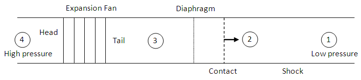Figure 3. Condition flow in sonic pipe

(32)

(33)

Also temperature and density for the zone 2 can be obtained by vertical shock relations. In zone3 we have:

(34)

Also, because the transition between zones 3 and 4 is isentropic, other variables in zone3 can be calculated by knowing the conditions in zone4. The characteristics theory should be used for expansion zone. Based on this theory, we have:

(35)

Parallel to each wave also we have:

(36)

Using these equations, the fluid velocity along each characteristic in the expansion zone is calculated by the following equation.

(37)

Having velocity, other variables can be obtained by characteristic equation and isentropic equations for perfect gas. For example, the sound velocity is:

(38)

Velocity is function of x, and thus sound velocity or temperature at each position can be calculated. Also, for calculation by the above equations, the following constraints govern.

(39)

Thus by choosing of initial conditions, analytical solutions for the desired time is obtained from the above equations.

5.2. Physical Conditions of Sonic Pipe

For calculating Sonic Pipe, by TVD and ACM methods, a specific geometry by defined initial conditions is used. Initial conditions are given in Table 1, The used gas has properties 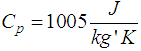, γ=1.4 and general parameters are as follow.

Sonic pipe length=10m

The membrane location: Pipe center

The number of nodes, , 4 nodes in the direction y and 102 node in the x direction or Pipe Length

Time step:

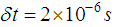Time Comparison =

Table 1. Initial conditions in sonic pipe

5.3. Numerical Solutions Comparison

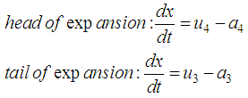
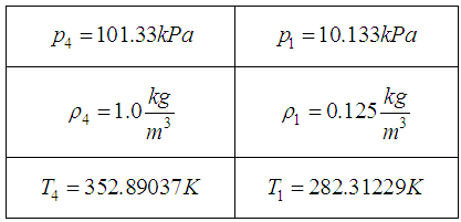
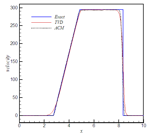
The results of numerical solution with TVD and ACM methods and with analytical solution are shown in Figures 4 to 7. In Fig. 4 to 7, velocity distribution figure, dimensionless pressure, dimensionless density and Mach number, by TVD method and by min mod limitation and also by reducing the numerical diffusion by ACM method, are shown respectively. In the ACM method the ω coefficient which is the Harten switching coefficient, for linear characteristic 3.0, and for non-linear characteristic 2.6 is selected.

As can be seen, TVD numerical diffusion in areas with extreme changes is great and capturing discontinuity is relatively weak. By applying ACM method, limitation property is enhanced and with lower numerical diffusion captures the discontinuities. In general, based on the results it can be seen that in the ACM method, capturing expansion waves is ideal and consistent with the analytical solution and also capturing the contact discontinuity which is available in the density distribution and Mach number figure, have significantly improved. The velocity figure in the calculated nodes is shown Fig 8.

Considering the figure, in the ACM method, shock wave is captured in fewer points rather than TVD method. As a result, by applying this method the shock wave capture is improved. So, it can be said that with increasing accuracy of the cell surface approximation, and also by calculating mass flux through ACM method, a drop in numerical diffusivity in PISO algorithm is evident.

Figure 4. Velocity distribution along Pipe

Figure 5. Dimensionless pressure figure

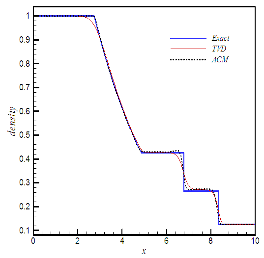Figure 6. Dimensionless density figure

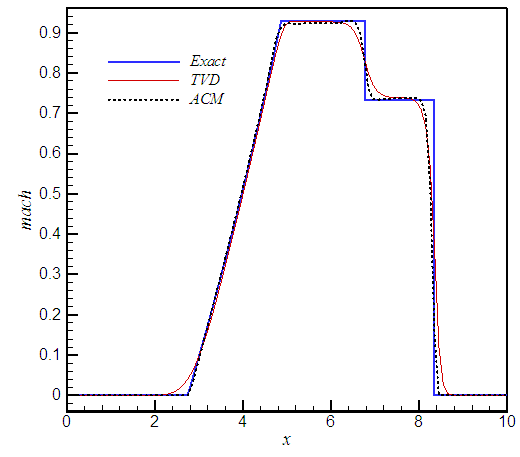Figure 7. Mach number figure

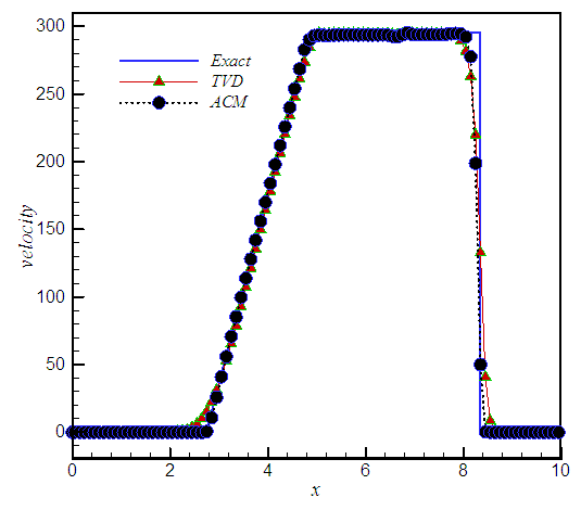Figure 8. Velocity figure in the calculated nodes

6. Conclusions

According to the contents of this paper discussed about compressible flow solutions by applying ACM method, to pressure-based algorithm, the results obtained from the present work can be summarized in several parts as follows:

1-The obtained results of ACM method in pressure-based algorithm, had an acceptable agreement with the obtained results of the density-based algorithm, and in some cases it was more accurate.

2-Due to extreme changes on both sides of the shock wave, one of the limitations of pressure-based algorithm was converging to the high order accuracies, which in this study this limit, is partly fixed. This convergence improvement may be due to different approach in calculating and analyzing the eigenvectors, eigenvalues and passing fluxes through diagonal surfaces to the components of original coordinates.

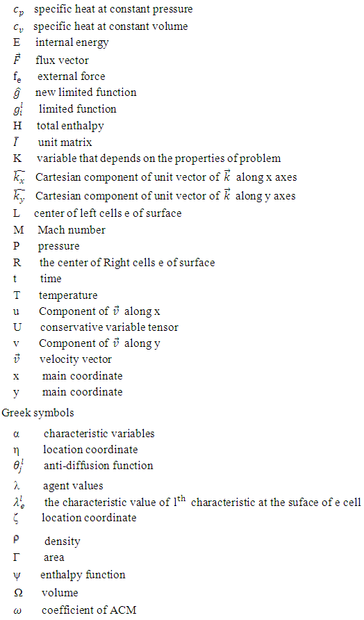
7. Nomenclature