N. K. Depuru Mohan 1, K. R. Prakash 2, N. R. Panchapakesan 3
1Department of Engineering, University of Cambridge, Cambridge CB2 1PZ, United Kingdom
2Division of Engineering, TATA Consultancy Services, Bangalore, India
3Department of Aerospace Engineering, Indian Institute of Technology Madras, Chennai, India
Correspondence to: N. K. Depuru Mohan , Department of Engineering, University of Cambridge, Cambridge CB2 1PZ, United Kingdom.
| Email: |  |
Copyright © 2015 Scientific & Academic Publishing. All Rights Reserved.
Abstract
A numerical investigation of multiple lobed jets was performed using the standard k - ε turbulence model. The present work laid emphasis on understanding the mechanism of mixing enhancement by multiple lobed jets. Further studies were carried out to compare mixing performance of multiple lobed jets with that of multiple conventional round jets for the same amount of momentum flux provided at the nozzle inlet. The numerical predictions matched reasonably well with the experimental data. The centreline velocity decay rate was fastest in the case of multiple lobed jets. The strongest streamwise vortices were generated in the case of multiple lobed jets. A passive scalar (temperature) was used for the quantification of mixing to figure out the jet configuration that provides the best mixing. In the near field of the jet, multiple lobed jets performed the best mixing by early introduction of strong streamwise vortices; while in the far field of the jet, both jet configurations behaved in a similar way.
Keywords:
Mixing augmentation, Multiple lobed jets, Multiple Round jets and turbulence modelling
Cite this paper: N. K. Depuru Mohan , K. R. Prakash , N. R. Panchapakesan , Mixing Augmentation by Multiple Lobed Jets, American Journal of Fluid Dynamics, Vol. 5 No. 2, 2015, pp. 55-64. doi: 10.5923/j.ajfd.20150502.03.
1. Introduction
The physics of mixing is of great interest in both fundamental and applied research. The process of mixing governs the amount of energy released in combustion chambers, the jet noise level of airplanes etc. More attention was paid to augment mixing in order to get beneficial end results such as increasing combustion efficiency, reducing jet noise, reducing NOX emissions etc. A lobed nozzle has circular cross-section at the inlet and a convoluted shape at the exit. It generates strong streamwise vortices at the nozzle exit itself thereby enhancing the near-field mixing. Vortex enhanced mixing has become one of the highly focused research areas in recent years. Lobed nozzles are primarily used in jet engines for suppressing the jet noise. Other applications of lobed nozzles are increasing propulsion efficiency and thrust augmentation. A multiple jet configuration is the one in which two or more number of jets is discharged from the same exit plane and separated by a finite distance. One of the major applications of multiple jets is to augment mixing. On the other hand, it reduces the jet noise level thus assisting in compliance with stringent noise regulations. Many high performance aircrafts such as F-15, B-1B use multiple jet configurations. Sometimes, these aircrafts are operated in assisted takeoff mode with a booster rocket under the wing for a takeoff from smaller runways. Multiple jets are used in the exhaust plumes from a rocket thruster with strap-on boosters. Multiple jets in cross flow are commonly used in film cooling of combustion chamber walls, turbine blades and reentry vehicle nose cones. Multiple jets are used in micro-blowing technique for the reduction of skin friction drag. Multiple jets are also used in electro spinning technique to increase the production rate of polymer nanofibers.
1.1. Salient Features of a Subsonic Turbulent Free Jet
Consider a turbulent jet issuing from nozzle, with a uniform velocity as shown in the figure below, into an infinite fluid at rest, both fluids being of same density. A subsonic turbulent free jet (as shown in figure 1.1) is divided into three principal regions: core, transition and fully developed region. The core region in the jet has a constant velocity and very little turbulence, where as outside the core region, the mean velocity decreases outward in the shear layer region and the flow is highly turbulent. The transition region is accompanied by a sharp change in the centreline velocity with the axial distance. In fully developed region, the jet becomes self-similar i.e. profiles of the normalized flow variables such as mean velocity, turbulence intensity etc. become similar at various axial locations.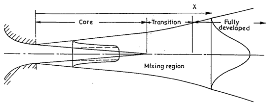 | Figure 1.1. Salient features of a subsonic turbulent free jet |
1.2. Jet Flow Control Techniques
Jet flow control has applications in combustion, aerodynamic noise, and jet propulsion. In general, flow control involves passive or active devices to effect a beneficial change in wall bounded or free-shear flows. Whether the task is to delay/advance transition, to suppress/enhance turbulence or to prevent/provoke separation, useful end results include drag reduction, lift enhancement, mixing augmentation and flow-induced noise suppression. The jet flow control techniques are broadly classified into two categories: active and passive. Active jet flow control affects the flow evolution properties by introducing externally powered perturbations into the jet flow e.g., blowing, suction, zero momentum flux etc. Passive jet flow control affects the flow evolution properties by changing the geometry of nozzle e.g., tabbed nozzle, chevron nozzle, lobed nozzle etc.
2. Literature Review
Paterson (1982) was the first to measure the velocity and turbulent characteristics downstream of a lobed nozzle/mixer. He concluded that a lobed nozzle/mixer could cause large-scale streamwise vortices of alternating sign, which are believed to be primarily responsible for the enhancement of mixing. Werle et al (1987) and Eckerle et al (1990) suggested that the process of formation of the large-scale streamwise vortices is an inviscid one, which was proposed to take place in three basic steps: vortices form, intensify and rapidly break down into small-scale turbulent structures. Elliott et al. (1992) found that both the streamwise vortices shed from a lobed trailing edge and the increase in initial interfacial area associated with the use of lobe geometry are significant for increasing the mixing compared with that occurring within a conventional flat plate splitter. McCormick and Bennett (1994) revealed that the interaction of Kelvin-Helmholtz (spanwise) vortices with the streamwise vortices produces the high levels of mixing. The streamwise vortices deform the normal vortices into pinch-off structures and increase the effect of stirring in the mixing flow. These effects result in the creation of intense small-scale turbulence and mixing. Ukeiley et al. (1992, 1993) and Glauser et al (1996) suggested that the turbulence dominated mixing in the lobed mixer flow field is due to the collapse of the pinch-off shear layer. The collapse of the shear layer onto itself, which occurred at a distance downstream of 3-6 times the lobe height, induced a burst of energy characterized by a region or pocket of high turbulence intensity. Belovich and Samimy (1997) summarized the results of previous research by stating that the mixing in a lobed nozzle/mixer is controlled by three primary elements. The first is the streamwise vortices generated due to the lobed shape, the second is the increase in interfacial area between the two flows due to the special geometry of lobed structures and the third is the Brown–Roshko type structures which occur in any shear layer due to the Kelvin–Helmholtz instabilities. Hu et al. (2001, 2002) suggested that the lobed jet mixing flow has a shorter laminar region, a smaller scale of the spanwise Kelvin–Helmholtz vortices, earlier appearance of small-scale turbulent and vortical structures and larger regions of intensive mixing in the near field of the jet flow. Cooper and Merati (2005) have done numerical simulation of a single lobed jet and they concluded that the realizable  turbulence model predictions are closer to the experimental data.Not much research has been carried out on experimentation or computation of multiple lobed jets. The present study will emphasize on the mixing and flow characteristics of multiple lobed jets. The objective of the present study is to compare the mixing performance of multiple lobed jets and multiple round jets. Firstly, the numerical simulation of a single lobed jet will be performed and then it will be compared with the prior published experimental results. Secondly, the numerical simulation of multiple lobed jets will be done and then to compare their mixing performance with that of multiple conventional round jets in order to find out a jet configuration that performs the best mixing.
3. Lobed Mixers and Streamwise Vorticity Generation
The lobed nozzle/mixer (as shown in figure 3.1) has a circular/flat cross-section at the inlet and a convoluted shape at the exit as shown in the figure. The outer penetration angle of the lobed nozzle was kept less than 7 degrees to avoid flow separation. In the present study, a six lobed nozzle was used as it was found to be more efficient during the optimization of the geometry of lobed nozzle for better mixing. Lobed mixers are well suited to the study of mixing augmentation because they allow the controlled introduction of streamwise and transverse vorticity along the interface between co-flowing streams. In a lobed mixer, the generation of streamwise vorticity is associated with the variation in aerodynamic loading along the span of the mixer. At the trailing edge, a continuous distribution of streamwise vorticity (as shown in figure 3.2) is discharged into the flow, evolving downstream into an array of discrete counter-rotating vortices. The vortices grow through turbulent diffusion and the circulation eventually decays as the counter-rotating vortices diffuse into one another. The streamwise vortices downstream of such forced mixing devices are typically larger, in both magnitude and scale, than those in naturally developing free shear layers and boundary layers.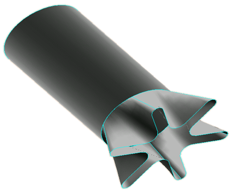 | Figure 3.1. Lobed nozzle geometry |
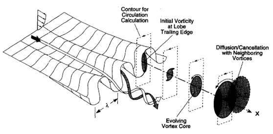 | Figure 3.2. Generation of streamwise vortices by a lobed mixer (Waitz et al. (1997)) |
The important vortical elements in the downstream flow field are as shown in figure 3.3. The counter-rotating pairs of streamwise vortices are the largest scale structures in the flow for three to ten lobe wavelengths downstream. There are also transverse vortices associated with the instability of the shear layer between the two streams of different velocity on either side of the plate. The difference in scale between streamwise and transverse vortices allows adoption of a simplified view of the principal mechanisms for interaction between the two structures. In this view, transverse vorticity is associated with turbulent transport which diffuses streamwise vorticity across the symmetry planes between the counter-rotating streamwise vortices, thereby reducing the magnitude of the streamwise circulation. The streamwise vortices produce stretching along the axes of the transverse vortices. 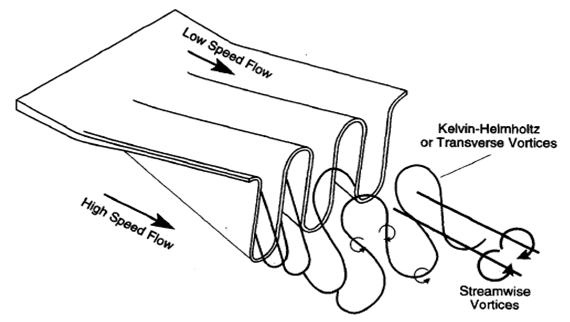 | Figure 3.3. Streamwise and transverse vortices generated by a lobed mixer (Waitz et al. (1997)) |
4. Vortex-Enhanced Mixing
In this section, the mechanisms responsible for mixing enhancement in lobed jet flows are discussed. When an interface between two fluids of different properties (e.g. chemical composition, momentum or energy) is convected in the velocity field of a vortex, the stretching of the interface creates two interrelated effects. The first is an increase in interfacial surface area and the second is an increase in the magnitude of gradients normal to the interface. Both these effects augment mixing.With no strain, the mixing process is pure diffusion. Strain enhances the reaction rate by increasing the interfacial area and increasing gradients in the diffusion zone. Mixing augmentation in a vortex field is due to the same physical effects, but in a geometrically more complex situation. The vortex increases the interfacial length roughly linearly with time. This stretching of the interface is the principal agent for mixing augmentation.
5. Quantification of Mixing
The mixture is been described in a vague manner, as there is no one common definition for what is called a good mixture. Generally, a good mixture is the one that is ready for its intended duty in the earliest possible time. A pigment is well mixed with a bulk product when eye can no longer detect the color variation within the mixture. However, a magnifying glass may turn the previously satisfactory mixture into an unsatisfactory one. Hence, it is essential to fix a scale for viewing before assessing the quality of a mixture.In the present study, a mixture that needs to be quantified is a fluid-fluid mixture i.e. an air jet emerging into an ambient environment. Generally, to quantify mixing, scalars like species, temperature, dye etc. are used. Their distribution will indicate the quality of mixing. A statistical quantity like standard deviation is widely used to study the distribution of these scalars. In the present study, temperature is used as a passive scalar to quantify the mixing. As it is a passive scalar, it will not affect the flow dynamics of the jet. This is achieved by raising the temperature of the jet fluid by 5 K compared to that of the ambient air. An area-averaged standard deviation ‘σ’ of the temperature field is defined as: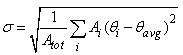 | (5.1) |
The distribution of the temperature field was assessed to quantify the mixing i.e. if the standard deviation of the temperature field is a low value then it implies that the mixing is done well.
6. Flow Modelling
The flow modelling involved the following steps:• Modelling the domain and generate the mesh using HyperMesh. • Check for quality of the mesh such as aspect ratio, jacobian etc.• Export the FEA model (called so in HyperMesh) to GAMBIT.• Check for quality of the imported model and the mesh.• Specify the nature of Boundary conditions.• Export the model to FLUENT.• Check for quality of model in FLUENT.• Specify the initial values of boundary conditions.• Specify the turbulence model and the limits of residuals for convergence.• Solve the flow equations. A pre-processing tool, GAMBIT, is supplied along with the commercial fluid flow solver, FLUENT, which is used to build and mesh the computational domain. In addition, HyperMesh is used due to the complexity involved in the modelling of multiple lobed jets. The boundary conditions of the computational domain are shown in figure 6.1 and the generated mesh is shown in figure 6.2. 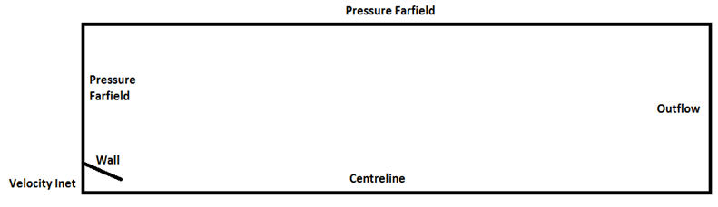 | Figure 6.1. Boundary conditions of the computational domain |
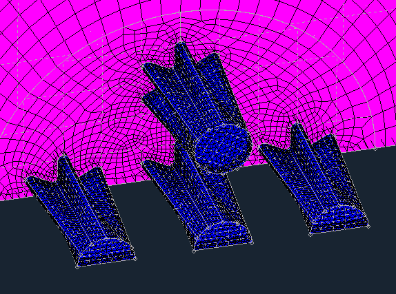 | Figure 6.2. Generated mesh for the computational domain |
6.1. Standard k-ε Turbulence Model
The standard  turbulence model (proposed by Launder and Spalding) is a semi-empirical model based on model transport equations for the turbulence kinetic energy (k) and its dissipation rate
  The model transport equation for k is derived from the exact equation, while the model transport equation for
  was obtained using physical reasoning and bears little resemblance to its mathematically exact counterpart. In the derivation of the
  model, it was assumed that the flow is fully turbulent, and the effects of molecular viscosity are negligible. The standard
  model is therefore valid only for fully turbulent flows.The turbulence kinetic energy, k, and its rate of dissipation,
  are obtained from the following transport equations:
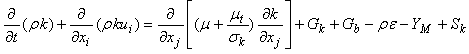 | (6.1) |
and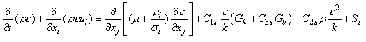 | (6.2) |
In these equations, Gk represents the generation of turbulence kinetic energy due to the mean velocity gradients. Gb is the generation of turbulence kinetic energy due to buoyancy. YM represents the contribution of the fluctuating dilatation in compressible turbulence to the overall dissipation rate.  and
and  are constants.
  and
and  are the turbulent Prandtl numbers for k and
  , respectively.
  and
and  are user-defined source terms. In this study, the jet flow is non-buoyant and incompressible. Therefore, Gb and YM are set to zero. For the standard
  model,
  and
and  are also set to zero.
6.1.1. Modelling the Turbulent Production
The term Gk, which represents the production of turbulence kinetic energy, is modelled identically for the standard, RNG, and realizable  models. From the exact equation for the transport of k, this term may be defined as
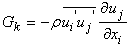 | (6.3) |
To evaluate Gk in a manner consistent with the Boussinesq hypothesis, | (6.4) |
where R is the modulus of the mean rate-of-strain tensor, defined as | (6.5) |
6.1.2. Modelling the Turbulent Viscosity
The turbulent (or eddy) viscosity  is computed by combining k and
  as follows:
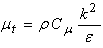 | (6.6) |
where  is a constant.The model constants
  and
and  have the following default values:
 and
and  These default values have been determined from experiments with air and water for fundamental turbulent shear flows including homogeneous shear flows and decaying isotropic grid turbulence. They have been found to work fairly well for a wide range of wall-bounded and free shear flows.
6.2. Flow Conditions
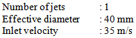
6.2.1. Single Lobed Jet
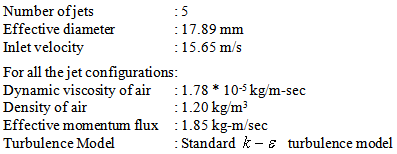
6.2.2. Multiple Lobed/Round Jets
7. Results and Discussion
A single lobed jet flow was simulated and then numerical results were validated with the experimental data (Hui Hu et al. (2001 & 2002)). Figure 7.1 show that the  model over-predicts the centreline velocity decay. The maximum difference between
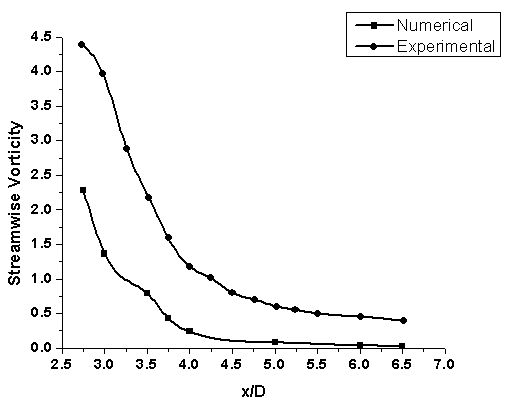
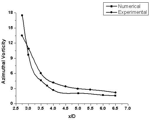
  predictions and experimental data was around 13%, which can be considered as a good prediction in turbulent flows. Figures 7.2 and 7.3 show that it under-predict the streamwise and azimuthal vorticity. Though it is not able to capture the streamwise vorticity that good, the prediction of azimuthal vorticity was closer to the experimental data. The equation of the streamwise vorticity revealed that the important contribution to the streamwise vorticity decay rate is the secondary shear stress and the normal stress anisotropy. Neither is well predicted by
  model, leading to poorer predictions of the streamwise vorticity decay rate. However, the trend of streamwise vorticity decay along the axial distance is very well predicted by the turbulence model.
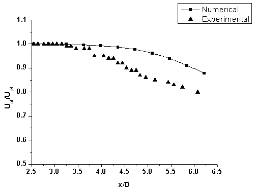 | Figure 7.1. Centreline velocity decay |
 | Figure 7.2. Streamwise vorticity |
 | Figure 7.3. Azimuthal vorticity |
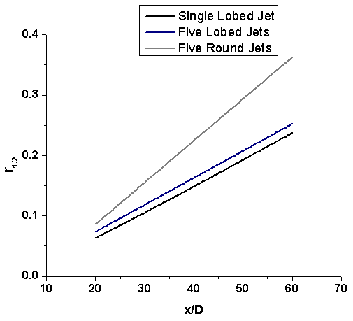
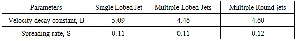
A grid independence study was performed by varying the number of elements in the computational domain from 2x10⁵ to 4x10⁵. The maximum difference in numerical results was about 2% between 3x10⁵ elements and 4x10⁵ elements computational domain. Hence, an optimum computational domain of 3x10⁵ elements was chosen for the numerical simulations in the present study.Figure 7.4 shows the variation of centreline velocity decay for the jet configurations i.e. single lobed jet, multiple lobed jets and multiple round jets. Assuming self-similarity in the zone of established flow downstream of the potential core, the integral model shows that the centreline velocity exhibits an inverse dependence on the axial distance, x. The centreline velocity decay is a good indication of mixing. Faster the centreline velocity decay, better the mixing is. From the plot, it is clear that the centreline velocity decay is faster in the case of multiple lobed jets thereby performing the mixing more effectively. Figure 7.5 shows the spreading rate for different jet configurations. The theory says that the spreading rate varies linearly with the axial distance, x. It was found that spreading rate is slightly more in the case of multiple round jets whereas the velocity decay is faster in the case of multiple lobed jets. The following table 7.1 shows the velocity decay constant, B and spreading rate, S for different jet configurations with the same momentum flux at the nozzle inlet.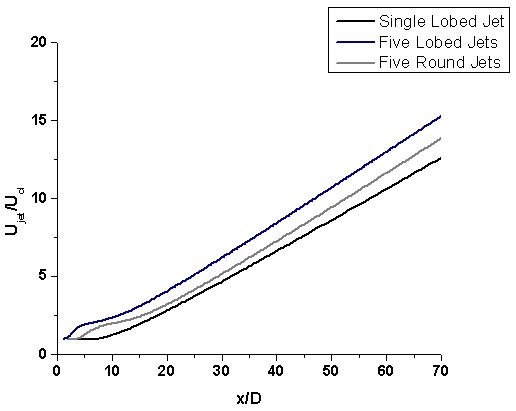 | Figure 7.4. Centreline velocity decay |
 | Figure 7.5. Spreading rate |
Table 7.1. The velocity decay constant, B and spreading rate, S for different jet configurations
 |
| |
|
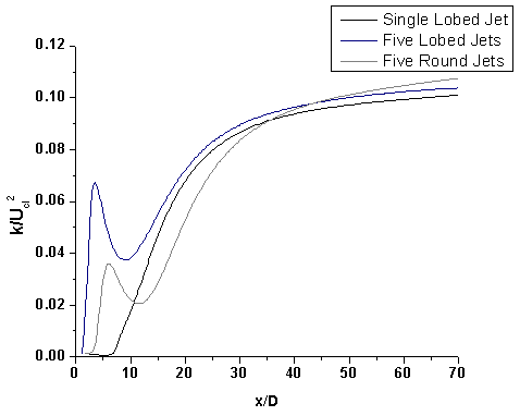
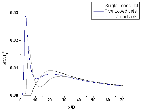
Figure 7.6 shows the radial plot of the normalized axial velocity at x/D=60. It was found that the velocity profiles of all jet configurations are similar at x/D=60. It implies that the first order quantities like velocities are similar in all jet configurations beyond x/D=60. Figure 7.7 and figure 7.8 show the variation of normalized kinetic energy and normalized dissipation along the axis of the jet. It was found that  is not similar even at x/D = 70 whereas
  becomes similar. Mixing enhancement could be achieved through high shear stress rates, high turbulence levels and strong streamwise vortices.
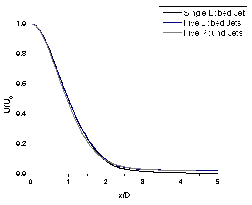 | Figure 7.6. Radial plot of normalized axial velocity at x/D=60 |
 | Figure 7.7. Normalized kinetic energy |
 | Figure 7.8. Normalized dissipation |
Figures 7.9 and 7.10 show the radial profiles of the normalized kinetic energy and normalized dissipation at x/D=60. In both plots, the different jet configurations did not reach self-similarity. 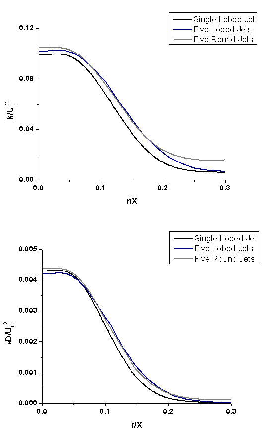 | Figure 7.9 and 7.10. Radial profiles of the normalized kinetic energy and normalized dissipation at x/D=60 |
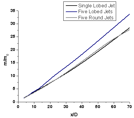
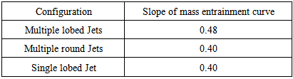
Figure 7.11 shows the plot of normalized radial velocity at x/D = 60. From this, it is clear that radial or entrainment velocity is more in the case of multiple lobed jets than in the case of single lobed jet. The entrainment velocity is inversely proportional to the radial distance from the jet centreline. The coefficient of proportionality increases in the zone of flow establishment and reaches a constant after the transition zone. It is suggested that the traditional definition of entrainment velocity, which maintains direct proportionality to the local jet velocity by the entrainment coefficient, should be augmented by this inverse function. Figure 7.12 shows the entrainment of ambient air into the jet along the downstream. It was found that the entrainment of mass is more in the case of multiple lobed jets. Table 7.2 gives the slope of the mass entrainment curve for different jet configurations. The slope of the mass entrainment curve is highest for the multiple lobed jets with a value of 0.48. This confirms that the amount of ambient air getting into the jet is highest in the case of multiple lobed jets because of its higher entrainment velocity.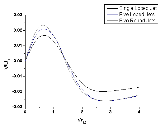 | Figure 7.11. Normalized radial velocity at x/D = 60 |
 | Figure 7.12. Mass entrainment curve |
Table 7.2. Rate of mass entrainment in different jet configurations
 |
| |
|
The temperature distribution will provide us both qualitative and quantitative information about the mixing performance by different jet configurations. For example, if the standard deviation of the temperature field is a low value then it implies that the mixing is done well. Figure 7.13 shows the standard deviation of the temperature field in the near field of jet. It was found that multiple lobed jets perform mixing more effectively than any other jet configuration in the near field. Figure 7.14 shows the standard deviation of the temperature field in the far field of the jet. It was found that all jet configurations behave in a similar way in the far field. Figures 7.15 and 7.16 show the temperature contours at x/D = 2.75 and 4 respectively. From these contours, it is very clear that multiple lobed jets perform the best mixing in the near field of the jet because of its early introduction of the strong streamwise vortices.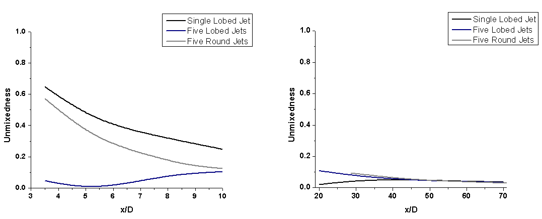 | Figure 7.13 and 7.14. Standard deviation of the temperature field in the near and far field of jet |
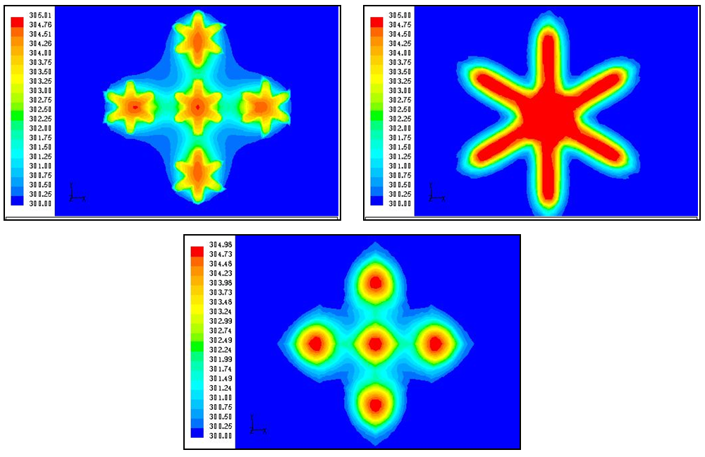 | Figure 7.15. Temperature contours at x/D = 2.75 for multiple lobed jets, single lobed Jet and multiple round jets (Range: 300 K – 305 K) |
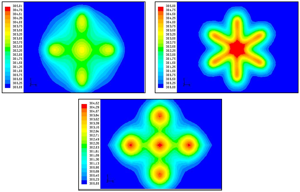 | Figure 7.16. Temperature contours at x/D = 4 for multiple lobed jets, single lobed jet and multiple round jets (Range: 300 K – 305 K) |
8. Conclusions
In this study, mixing augmentation by multiple lobed jets is numerically investigated. A one-to-one comparison of a single lobed jet and a single round jet is performed. Also, a one-to-one comparison of multiple lobed jets and multiple round jets is performed. It was found that the centreline velocity decay is faster in multiple lobed jets. In other words, the jet core length is shortest in multiple lobed jets thereby indicating its superior mixing capability. The first order quantities of all jet configurations have become similar beyond 30 jet diameters from the nozzle exit. But, the second order quantities have not become similar even at 60 jet diameters from the nozzle exit. The entrainment velocity is highest in multiple lobed jets, which draw more ambient air in to the jet thereby performing mixing effectively. Multiple lobed jets perform the best mixing in the near field of the jet (up to 5 jet diameters from the nozzle exit) because of its early introduction of the strong streamwise vortices. All jet configurations behave in a similar way in the far field of the jet (beyond 60 jet diameters from the nozzle exit). The lobed jets generate streamwise vortices, which mix the jet fluid and the ambient air more effectively. This concept of vortex-enhanced mixing seems to be promising. To achieve mixing augmentation, it is more efficient to have multiple small jets instead of a single big jet for the same momentum flux at the nozzle exit.
ACKNOWLEDGEMENTS
Authors acknowledge the TATA Consultancy Services Ltd, India for providing the computational facilities required to carry out the present work at their "Centre of Excellence in Computational Engineering" at the Indian Institute of Technology Madras, India.
Nomenclature
English Symbols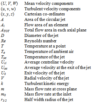 Greek Symbols
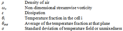
References
| [1] | PATERSON R. W. Turbofan mixer nozzle flow field - a benchmark experimental study. Transactions of the ASME, Journal of Engineering for Gas turbine and Power, 1982, 106, pp. 692-698. |
| [2] | ECKERLE, W. A., SHEIBANI, H., and AWAD, J. Experimental Measurement of the Vortex Development Downstream of a Lobed Forced Mixer. Transactions of the ASME, Journal of Engineering for Gas Turbine and Power, 1992, 114, pp. 63–71. |
| [3] | ELLIOTT, J. K., MANNING, T. A., QIU, Y. J., GREITZER, C. S., TAN, C. S., and TILLMAN, T. G. Computational and Experimental Studies of Flow in Multi-Lobed Forced Mixers. AIAA Journal, 1992, 92-3568. |
| [4] | McCORMICK, D. C., and BENNETT, J. C., Jr. Vortical and Turbulent Structure of a Lobed Mixer Free Shear Layer. AIAA Journal, 1994, 32, pp. 1852–1859. |
| [5] | UKEILEY, L., VARGHESE, M., GLAUSER, M. and VALENTINE, D. Multi fractal analysis of a lobed mixer flow field utilizing the proper orthogonal decomposition. AIAA Journal, 1992, 30, pp. 1260-1267. |
| [6] | UKEILEY, L. M., GLAUSER, M. and WICK, D. Downstream evolution of POD Eigen functions in a lobed mixer. AIAA Journal, 1993, 31, pp. 1392-1397. |
| [7] | GLAUSER, M., UKEILEY, L., and WICK, D. Investigation of Turbulent Flows via Pseudo Flow Visualization, Part 2: The Lobed Mixer Flow Field. Experimental Thermal and Fluid Science, 1996, 13, pp. 167–177. |
| [8] | BELOVICH, V. M., and SAMIMY, M. Mixing Process in a Coaxial Geometry with a Central Lobed Mixing Nozzle. AIAA Journal, 1997, 35, pp. 838-84l. |
| [9] | HU, H., KOBAYASHI, T., SAGA, T. and TANIGUCHI, N. A Study on a Lobed Mixing Flow by Using Stereoscopic Particle Imaging Velocimetry technique. Physics of Fluids, 2001, 13, pp. 3425-3441. |
| [10] | HU, H., SAGA, T., KOBAYASHI, T. and TANIGUCHI, N. Mixing Process in a Lobed Jet Flow. AIAA Journal, 2002, 40, pp. 1339-1345. |
| [11] | COOPER, N. J., MERATI, P., and HU, H. Numerical simulation of the vertical structures in lobed Jet mixing Flow. 43rd AIAA Aerospace Sciences Meeting and Exhibit, 2005, AIAA-2005-0635. |
| [12] | WAITZ, I. A., QIU, Y. J., MANNING, T. A., FUNG, A. K. S., ELLIOT, J. K., KERWIN, J. M., KRANSNODEBSKI, J. K., O’SULLIVAN, M. N., TEW, D. E., GREITZER, E. M., MARBLE, F. E., TAN, C. S., and TILLMAN, T. G. Enhanced mixing with streamwise vorticity. Progress in Aerospace Sciences, 1997, 33, pp. 323-351. |
 Abstract
 Reference
 Full-Text PDF
 Full-text HTML