1. Introduction

One of the problems related to computational methods is capturing the region with sharp gradients (sudden changes). This state occurs in flow when we encounter suddenly changes in flow variables. These kinds of changes are known as discontinuities. First-order approximation methods captured the sharp discontinuities with high error, while high-order shock-capturing methods are associated with non-physical fluctuations. For this purpose, the high-order methods without fluctuation (High Resolution Schemes) are designed in such a way to prevent the fluctuations, as much as possible, by having acceptable accuracy. The classical computational methods such as Jameson, TVD and ENO used in aerodynamic applications for computing compressible flows with shock waves are of these kinds. Since the basis of these methods is based on increasing the numerical dissipation in sudden and rapid changes in flow variables, so a relative decline will be observed in the accuracy said that the most important part of the finite volume method is calculating the passing flux through the cell of these regions. Considering that different characteristics have different dissipation from each other. The main important part of the finite volume method is calculation of the flux in the cell walls. Researchers have introduced a lot of methods for calculating these fluxes in a more accurate and low-cost way.

Godunov (1959) [1] for the first time used Riemann problem in the calculation of flux. Riemann problem is considered as a shock tube with two different pressures (two different speeds) that is separated by a diaphragm.

Godunov solved Riemann problem for each cell walls. In fact, Godunov method needs the answer of the Riemann problem, and in a practical calculation, this problem is resolved millions of times. The problem of Godunov method is the direct use of the Riemann problem with its complete solution that when the problem is resolved million times, the computing time greatly increases. Because of this reason, Roe (1981) [2] used the approximation method for solving the Riemann problem. Roe method is based on Godunov method. For this purpose, Roe used method of linear averaging, and this method is known as the Roe averaging method. After Roe, other people reform his method and different plans had been proposed based on Roe method. Jameson (1981) [3] used averaging and artificial viscosity method for calculating the flux. In this method, Jameson used modified Rung- kutta fourth order to discrete the time. The greatest advantage of this method in addition to simplicity and its use in complex geometries is its high resolution in capturing shock in transonic flows. The work of Jameson.et al was a combination of numerical dissipation of second and fourth order based on flow gradients that, with two adjustable parameters, was considered for central difference. Although considerable improvement was obtained in the results, but setting two parameters to extract acceptable results in discontinuities must be found by trial and error for each problem. In other words, the choice of optimal dissipation term depends on the experience of working with code. In addition, the direction of waves motion in the hyperbolic flow was overlooked. Harten [4] introduced total variation diminution (TVD) in 1984. In this method, having a reduction trait in total variations of conservation laws for both hyperbolic scalar equation and hyperbolic equations with constant coefficients were the main goals. One problem of TVD methods was that it changed to the first order methods in the discontinuities, therefore, smooth variations of solutions was created in the shock wave and other discontinuities. Note that, in the first order methods in which the second and higher derivatives of Taylor expansion are overlooked, diffusion errors were created and consequently the solution dispersed to the surrounding points. Another method that was proposed by Harten (1977, 1978) [5-6] for flows with discontinuities was the combination of a first order scheme with an ACM (Artificial Compression Method) switch.

In this method, ACM switch is operated as an artificial compression that appears in intensive gradients. Turkel et al (1987, 1997) [7] imposed a method called preconditioning to the density based algorithm, and showed that the usage of the new approach gave an aacceptable and accurate results of incompressible and small Mach numbers flows for solving compressible flow equations. Also in a recent study carried out by Razavi and Zamzamian (2008) [8], a new method based on density based algorithm and method of characteristics was presented by applying artificial compressibility method in order to solve incompressible fluid flow equations. Rossow (2003) [9] supposed a method to synthesize the density based and pressure based algorithms, which allows pressure based algorithm changes to the density based one. In this study, Riemann solver was studied in the incompressible flow regime, and solution algorithm is based on the pressure one. Synthesizing of this algorithm and density algorithm provides transition from incompressible to the incompressible flow regime, and it’s possible to solve both flows.

Colella and Woodward [10] implemented the idea of using both first-order flux and anti-diffusion term as a limiting flux. In this procedure, the calculated optimal anti-diffusion is added to the first order flux. Montagne et al (1987) [11] compared high resolution schemes for real gases. This comparison showed that approximated Riemann solvers were reliable for real gases. One of the main researches based on TVD idea was the Duru and Tenaud works [12]. In the Mulder and Vanleer (1985) [13] and Lin and Chieng (1991) [14] showed that the best variable in view of the numerical solution accuracy was the kind of variable by using the limitations on initial variables،conservative and characteristic which were experimented in the unsteady one-dimensional flow. Yee et al (1985) [15] developed first order ACM of Harten to TVD method with different approach. Thereby, instead of reducing degree in capturing shock waves، order of accuracy remained at an acceptable level and demonstrated relative favorable capturing of high gradients (Shock). In another research، Yee et al (1999) [16] directly imposed ACM switch to the numerical distribution term (filter) of TVD method. In this work, basic scheme namely the central difference term in the flux approximation at the cell surface was in order of two, four, and six. Also ACM terms were appeared in discontinuity locations. Thus, in that zones of flow without any discontinuity،Central Difference approximation was high and in exposing to the sudden changes in flow،numerical diffusion, which is less than the value of diffusion numerical second order TVD, are add to the Central difference term. Hatten (1983) [17] accomplished different designed in order to calculate and limit total amount of oscillation of variables or their error due to the idea of the total change (TVD).

2. The Basic Governing Equation

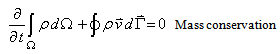
In this section, the mathematical formulating of the governing equations on compressible non-viscous flow used in all flow regimes and is known as Euler Equations, will be discussed. Euler equations for transiting flow from Ω volume and limited to Γ surface in the integral mode could be written as. Eqs. (1), (2), (3).

(1)

Momentum conservation:

(2)

Energy conservation:

(3)

That in the above equations, ρ is density, is the velocity vector, is the pressure, is external forces, E is internal energy and H is the enthalpy of the fluid that can be written as. Eq.(4).

(4)

The total internal energy of is defined as and in this equation e is defined as and is the specific heat at constant volume. The above equations could be defined in a whole and compressive way. So that if U represents a vector or tensor of conservation variables, represents conservation vector fluxes and is a unit matrix, then it can be written as .Eq.(5).

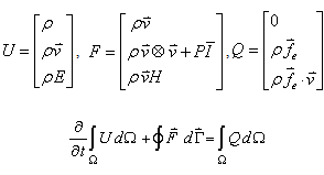(5)

If we write the above equation differentially and in vector mode, then we have. Eq.(6) as following:

(6)

In two-dimensional and unsteady flow, the Cartesian components of U vector and also F vector are defined by the following relations as. Eq.(7).

(7)

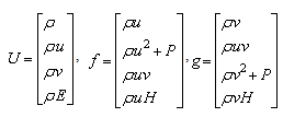
Where u and v are the components of velocity vector. In this case, equation (6) could be written in the Cartesian coordinate system as .Eq.(8).

(8)

The above equation is known as the Euler equation.

3. Calculating the Flux in Diagonal Surface

According to the practical problems, the computational grids are not always orthogonal, and grid lines are not along the flow; thus, the passing flux from the surface of cell could have component in both directions of x and y for each local direction; thus, changes must be created in the form of equations and the way of flux calculation to allow the calculations to be performed in non-orthogonal grids as well. In the most of researches conducted by Harten and Yee and other researchers, the method used frequently was finite difference, and computation was carried out in the computational grid which is different from physical grid; therefore, the matrix of left and right vectors and other flux parameters in the directions of Cartesian x and y have been used separately and unchanged. Finally, after calculations, conversion from local coordinates to the original coordinates would apply to them, but because at the present work the grid and discretization of governing equations are based on finite volume and computational grid is the physical grid itself, the considered method to calculate flux is based on the method of Hirsch (1990), and it is in the form that all flux sentences and its components at local directions of are decomposed to y and x components and added together.

For this task, it is necessary to investigate the grid geometry and the position of the cell surface to the adjacent cells centers. Geometry used in calculating the flux is shown in fig.1.

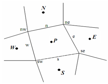Figure 1. Geometry used in calculating the flux

3.1. Calculating the Flux in the E Surface

In order to calculate the passing flux in the e surface of cell, the surface shown in the figure 1 is considered. If this surface is separately to be investigated, an arbitrary position of that surface in the locational coordinate (ξ,η) is related to the main coordinate (x,y) as figure 2.

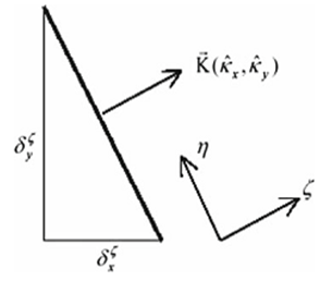Figure 2. Cell surface e in the local coordinates

The geometric relations for the above state could be written as .Eq.(9).

(9)

So, according to the symbols of figure 1, can be written as equation (10):

(10)

As it can be seen, and are the Cartesian components of unit vector of This unit vector is perpendicular to the surface of cell, and put along the locational direction. Noticing to the above equations, flux of velocity vector in direction can be defined as Eq.(11).

(11)

Conservative vector of variables is shown by and conservative vectors of mass flux, momentum and energy in each of adjacent cell center of e surface are as. Eq.(12).

(12)

Flux for each desired cell in e surface could be calculated as. Eq.(13).

(13)

In above equation, in hyperbolic equation system, for the two-dimensional flow four eigen values in above surface are as. Eq.(14).

(14)

“” sign means that matrix is defined at the surface of e cell, and all of its elements are based on Roe averaging method.

And also, the characteristic variable α in e surface from multiplying each row of the matrix of left special vector of in conservative variables could be calculated as .Eq.(15).

(15)

The above equations, in general and as a vector, could be written as .Eq.(16).

(16)

In these equations, subscript relations of are related to the center of left e cell and the center of right e cell surface, respectively. And also represents the row i of the left eigenvectors matrix. And in the relation (13) is the column i of matrix, as .Eq.(17).

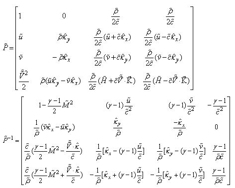(17)

Yee (1986) and Yee et al. (1999) proposed the following equation for diffusion sentence based on TVD approximation of (2^nd order –upwind TVD) the second order upstream method for local discretization as .Eq.(18).

(18)

Function has been suggested as .Eq.(19).

(19)

In the above equations, is eigen value related to lth characteristic in the surface of e cell and is the limiting function related to lth characteristic in the center of the ith cell, and is characteristic variable in surface of e cell that is equal to column l of matrix, and finally, function is entropy function. Harten and Hyman (1983) suggested the above condition as .Eq.(20).

(20)

That in this equation is zero for problems with moving shock waves is usually and is considered as a small amount for stationary waves. Different functions could be selected for limiter function of in the center of cell. Yee at al. (1999) proposed a number of these functions, and one of these functions is used in the present study which is as .Eq.(21).

(21)

Also, to avoid any problems in the implementation of the computer program, Yee et al (1999) introduced the following relations for the entropy and Gama functions as. Eq.(22).

(22)

Which in the all of computations was considered equal to , and was considered equal to .

In the present work in order to increase accuracy and reduce diffusion in the discontinuity another method had been considered for applying ACM to the TVD diffusion sentence.

Due to already mentioned reasons, ACM cannot be applied to the diffusion sentence directly, so instead of applying it directly to the TVD diffusion sentence, anti-diffusion function, which is located inside the diffusion sentence and affect it indirectly, has been applied to limiter function in this study. The applied method is as .Eq.(23).

(23)

As it could be seen, in the TVD diffusion sentence, g function is replaced by a new limiter function () which is based on above equation. In this equation is ACM coefficient, and since each numerical wave (linear and nonlinear waves) has diffusion germane to itself, so, we will have different coefficients for each characteristic. Anti-diffusion function of in i cell, for each l characteristic is defined as .Eq.(24).

(24)

Where α represents characteristic variables and will be calculated in cell surface. Also, is a coefficient that in addition to be different for different characteristics, is the function of the physics of the problem, and for any special flow it is different from the flow with other specification, so in the calculation for a particular flow, it would be obtained through the trial and error method. According to the above equations, the new limiting function of () would be greater than the limiting function of TVD method. As a result, regarding the limiter reinforcement, the possibility of increasing the accuracy and convergence of the solution exists which is effective in improving capture shock waves. However, with excessive increase of and consequently increase of the limiting function which will have excessive decline of diffusion with itself, there is the possibility of disturbance in the solution convergence process. Thus, in a specific flow for coefficient, an optimum range or value must be specified and those values must not be accompanied by increasing of accuracy and more reduction of convergence and increasing of calculation costs. This case, for each experiment, will be discussed in results section.

4. Results and Discussion

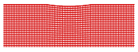
In this section, the obtained results from solving non-viscous flows by TVD, Jameson and TVD-ACM methods are presented. The obtained results from three methods of classic TVD, ACM, and Jameson are compared with each other. Also effect of dissipation coefficients, number of nodes, and variations of ACM coefficients are investigated on resolution of shock capturing and convergence. And the effect of reducing numerical dissipation on results will be discussed. The issue is steady and two-dimensional flow over an arc shape bulge of a circle (bump) at various Mach numbers in the supersonic regime that is an appropriate test in computational fluid dynamics for calculation compressible flow. Figure (3) shows the number of grid used on the channel including 120 in the horizontal direction and 40 in the vertical direction. Also figures (4), (5), (6) and (7) show Mach distribution on the upper wall, on the lower wall, pressure distribution on the lower wall, and pressure distribution on the upper wall respectively.

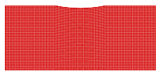Figure 3. Supersonic flow over 4% thick bump, inlet M=1.4 Supersonic bump geometry and 120*40 mesh

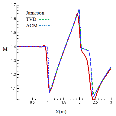Figure 4. Mach number on the upper wall inlet M=1.4

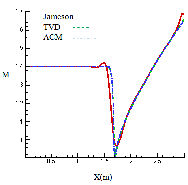Figure 5. Mach number on the lower wall inlet M=1.4

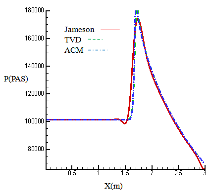Figure 6. Pressure on the lower wall inlet M=1.4

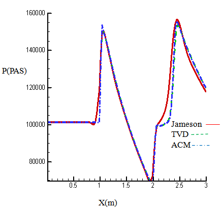Figure 7. Pressure on the upper wall inlet M=1.4

4.1. Supersonic Flow with Inlet Mach 1.4

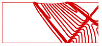
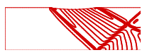
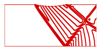
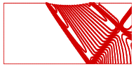
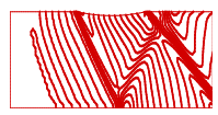
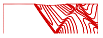
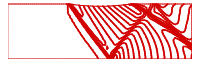
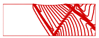
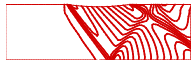
As figures (4) – (7) show, reducing numerical diffusion leads to the increment of the accuracy in calculating Mach number and pressure in places that wave reflection had occurred. For observing the increase of accuracy calculation in total calculation field, the figures related to Mach contours are shown in figures (8), (9), and (10).

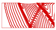Figure 8. Mach contours (Jameson) inlet M=1.4

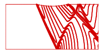Figure 9. Mach contours (TVD) inlet M=1.4

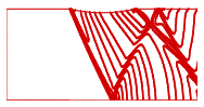Figure 10. Mach contours (TVD-ACM) inlet M=1.4

Also, pressure contours for Jameson, TVD and ACM methods in present research are shown in figures (11), (12), and (13).

Figure 11. Pressure contours (Jameson) inlet M=1.4

Figure 12. Pressure contours (TVD) inlet M=1.4

Figure 13. Pressure contours (TVD-ACM) inlet M=1.4

As we can see, in ACM method, all waves including shock waves dispersion, waves interaction, and reflection from the walls are better captured relative to the both TVD and Jameson methods.

4.2. Supersonic Flow with Inlet Mach 1.65

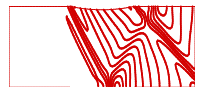
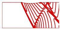
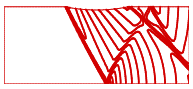
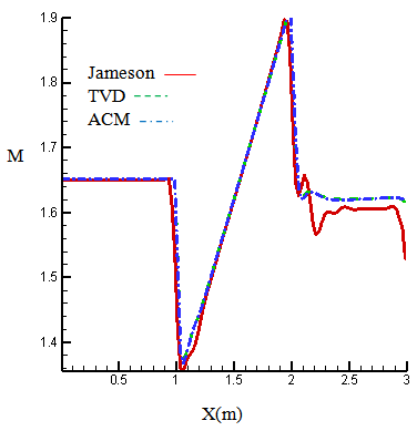
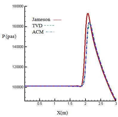
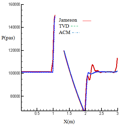
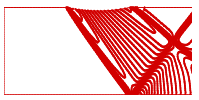
In this state, the channel dimensions, the grid type and the number of cells are the same as previous state and are according to figure (3), except that Mach number of inlet flow is greater than it. Figures (14) and (15) show the calculated results of Mach number distribution, and figures (16) and (17) show the distribution of dimensionless pressure in lower and upper boundary of the channel. Figures (18), (19) and (20) are related to Mach contours inside the channel, and figures (21) to (23) are also related to the results of pressure contours calculated by Jameson, TVD, and ACM methods in the present study.

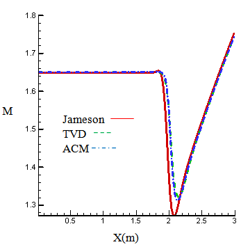Figure 14. Mach number on the lower wall inlet M=1.6

Figure 15. Mach number on the upper wall inlet M=1.65

Figure 16. Pressure on the lower wall inlet M=1.65

Figure 17. Pressure on the upper wall inlet M=1.65

Figure 18. Mach contours (Jameson) inlet M=1.65

Figure 19. Mach contours (TVD) inlet M=1.65

Figure 20. Mach contours (TVD-ACM) inlet M=1.65

Figure 21. Pressure contours (Jameson) inlet M=1.65

Figure 22. Pressure contours (TVD) inlet M=1.65

Figure 23. Pressure contours (TVD-ACM) inlet M=1.65

As the results show, although the base density algorithm is appropriate for calculating compressible flow, but figure (18) does not represent a very acceptable capturing of the shock waves. Also at the exit of the channel, due to lack of appropriate boundary condition or its low order, fracture is observed in outlet wave, and also clearness and capturing of reflective wave from the lower wall is weak. According to the figures (18), (19), (20) and also figures (21), (22) and (23) related to pressure contours, it can be seen that in this study the problem of fracture of waves at outlet boundary in TVD and ACM methods is solved, and also all of the waves include the diffusion of shock waves, reaction of waves together and reflection from walls had been captured with the better quality than pervious works. Now, in order to study the influence of the number of grid nodes on resolution of shock capturing and convergence, a grid with 90*30 dimensions are used. Then Mach contours for the three methods (Jameson and TVD and ACM methods) are illustrated. In figure (24), the grid used on the bump is shown, and in figures (25), (26), and (27) contours of Mach number for three mentioned methods are shown.

Figure 24. Supersonic flow over 4% thick bump, inlet M=1.4 Supersonic bump geometry and 90*30 mesh

Figure 25. Mach contours (Jameson) inlet M=1.4

Figure 26. Mach contours (TVD) inlet M=1.4

Figure 27. Mach contours (TVD-ACM) inlet M=1.4

As it can be seen, with increasing in the number of grids, time of computations is increased to reach the convergence limitation. Also quality of shock waves capturing is increased. But the size of grids should not be so small because time of calculations and number of iterations are increased; and subsequently the stability of the solutions are affected. Now, the effect of the dissipation coefficients on resolution of the shock capturing and convergence are to be investigated. It’s obvious that the dissipation coefficients in the Jameson method are shown by and Therefore, we use a grid with dimension of 80*20. 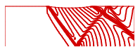In Jameson method, and . In figures (28), (29), and (30) contours of Mach number by variation of dissipation coefficients are shown.

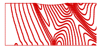
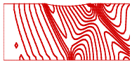
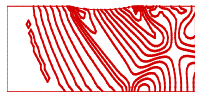Figure 28. Mach contours (Jameson) inlet M=1.4

Figure 29. Mach contours (Jameson) inlet M=1.4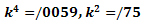

Figure 30. Mach contours (Jameson) inlet M=1.4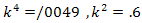

These figures (28), (29) and (30) show that with increment of the artificial viscosity, solution is more stable, and accuracy of the shock capturing is decreased. Reversely, with decrement of the artificial viscosity, solution is become more unstable and linear instability is occurred. Now, shock wave capturing is investigated in bump channel with grid dimensions of 90*30. All parameters such as values of boundary condition, size of grid for calculation of different variables of flow are the same previous values except that in the ACM method, anti-diffusion function with different coefficients is imposed. According to contours of Mach number shown in figures (31), (32) and (33), it’s concluded that the stability of results can be affected by reducing coefficients. Also, ACM coefficients for nonlinear fields should be less than those for linear fields in order to stabilize the solution. Changing of ACM coefficients in quality of shock waves capturing has a negligible effect according to the contours of Mach number.

Figure 31. Mach contours (ACM) (.6,.3)

Figure 32. Mach contours (ACM) (.7,.7)

Figure 33. Mach contours (TVD-ACM) (.27,.5)

4.3. Comparison of the Convergence of the Solution and Calculation Cost under the Influence of Various Parameters

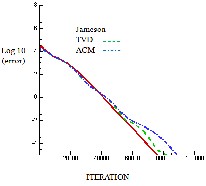
In this part of the present study, the convergence process of solution and calculation cost in numerical experiments related to supersonic flows in bulge of the bump for convergence curves that had been compared for each specific flow are discussed. The only difference is just in applying anti-diffusion function with different coefficients for ACM method, and other calculation parameters such as amounts related to boundary conditions and the grid size for calculating different variables of flow are the same. In figure (34), convergence diagram for velocity component in supersonic flow with incoming Mach 1.65 is shown. As it can be seen in figure (34), by choosing ω=.6 and ω=.3 for linear and nonlinear fields, convergence is to be improved.

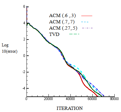Figure 34. Residual history of velocity "u" for M=1.65. The numbers in parenthesis (.6,.3) and (.7,.7) and (.27,.5) correspond to (ω1,2,ω3,4) for ACM, where ω1 and ω2 are considered for linear and ω3 and ω4 for nonlinear scopes

Therefore, it could be stated that by increasing ACM coefficient, diffusion in the capturing of discontinuous decreases and quality of capturing will be better, but it cannot be claimed that convergence would be better in this condition, because reducing numerical diffusion has excessively a negative impact on the convergence process and it will disrupt it. Therefore, for having the best convergence, it is necessary to find optimum values for the coefficients of anti-diffusion function in each particular flow by using trial and error method. In the relative coarse grids, ACM coefficients should be smaller for non-linear fields relative to the linear fields for stabilizing the solution. Hereby, numerical dissipation for stability of solutions and reduction of iterations due to the reducing in the number of cells are satisfied simultaneously; therefore, solution can better converge. Now in this section, convergence diagram related to the variation of artificial dissipation coefficients for 80*20 grid with considering Mach 1.4 at inlet is shown in figure (35). It’s concluded that the stability of solutions is affected by reducing these coefficients. Also, number of iterations and consequently the needed time for converging to steady state are increased by increment of these coefficients. Solution becomes more stable and accuracy of shock capturing is decreased with increment of the artificial viscosity. Reversely, with decreasing the artificial viscosity, the solution become unstable and linear instability is occurred. In figures (36) and (37), convergence diagrams for two specified grids are shown.

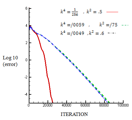Figure 35. Convergence diagram related to the variation of artificial dissipation coefficients for 80*20 grid with considering Mach 1.4 at inlet

Figure 36. Residual history of velocity "u" for M=1.65.(120*40)

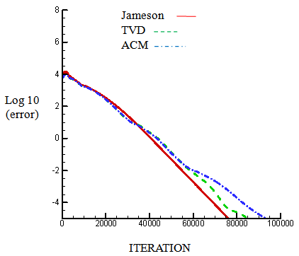Figure 37. Residual history of velocity. "u" for M=1.65.(90*30)

As it can be seen in two figures (36) and (37), although two grids have different nodes, the number of iterations is equaled together while the time of computations is more in the finer grid (120*40) as a result of cells number.

5. Conclusions

According to the mentioned points in this section about solving compressible flow by applying TVD and ACM methods to the density-based algorithm, the results obtained of the present study are summarized as following:

1- By applying the methods of ACM and TVD to the density-based algorithm, the limitations of using this algorithm and extending it in compressible regimes in terms of capturing accuracy of particle waves will be relatively resolves.

2- The velocities of characteristic became more converged due to the reinforcement of the limiter. Thus, for an algorithm of the same solution, TVD and ACM methods show better capturing and clearness of the shock waves than Jameson method in the indicated conditions such as simple waves, wave’s reflection and the interaction of waves with each other.

3- In the present study, the quality of capturing shock waves by TVD method, after ACM method, has considerable improvement compared with other published results related to density-based algorithm.

4- In this study, not only the quality of capturing discontinuities in total flows had been improved by applying ACM and TVD methods, but also, the improvement of the convergence of the solution process and also the reduction of calculation cost in supersonic flow is considerable as well.

5- In density based algorithm, with increasing the number of grids, solution converges faster and quality of shock waves capturing is increased.

6- By reducing coefficients of artificial dissipation, stability of solutions is affected. Also by increasing these coefficients the number of iterations and time of calculations for reaching to the steady state is increased.

7- Solution becomes more stable and precision of shock capturing is decreased with increment of the artificial viscosity. However, with reducing the artificial viscosity, the solution become unstable and linear instability is occurred.

8- In the relative coarse grids, in order to stabilize the solution and improvement of solution convergence, ACM Coefficients should be less in the nonlinear field than linear field. Therefore, in addition to satisfying the enough numerical diffusion for stability of solution, decrement of cells reduces iterations, and subsequently convergence of solution is improved.

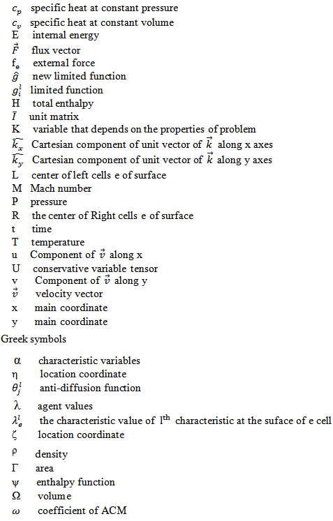
Nomenclature