1. Introduction

One problem of computational methods is capturing the zone with high gradient. This is when step variations are occurred in the flow variables which are known as discontinuities. The first order approximation methods capture the sharp discontinuities with significant errors while high order methods capture these regions with non-physical oscillations. Therefore, the high order methods without oscillations have been designed in the way that refrain the oscillations of solutions in addition to have a high accuracy. The classic computational methods such as TVD, Jameson, ENO, and etc. are categorized in these methods that applied in aerodynamic, especially compressible flows with shock waves. Whereas these methods are based on the increment of numerical diffusion in the sudden variations of flow variable, the accuracy of solutions is decreased in these regions. The main important part of the finite volume method is calculation of the flux in the cell walls. Researchers have introduced a lot of methods for calculating these fluxes in a more accurate and low-cost way. In the first time, Godunove [1] used Riemann solution for computing the flux in 1959. Riemann solution was defined as a shock tube with two different pressure (or velocity) which was apart by a diaphragm. Godunov solved Riemann equation for each cell wall. In fact, the Godunov method required the solution of Riemann equation, and solved this equation in an actual computation, continuously (about million times). The problem of Godunov method was the direct usage of Riemann equation with its exact solution that increased the time of calculations remarkably when it was solved million times. For this reason, Roe [2] used an approximate method based on the Godunov method for solving the Riemann equation in 1981. Roe used an interpolating approach for linearizing called Roe interpolation method. Then, many researchers modified this method and suggested different methods based on Roe method. Jameson [3] in 1981 used both interpolation and artificial viscosity methods to calculate the flux. Jameson used the modified fourth order Rung-Kutta method for time discretizing. Using in the complex geometries, good accuracy in capturing the shock in transonic flows, and simplicity were the main advantages of this method. Jameson et al. work was a synthesizing of second and fourth order numerical diffusion based on the flow gradients that considered with two adjustable parameters for central difference. Although a considerable improvement was observed in the results, these two parameters should be adjusted with the trying-error procedure for obtaining acceptable results in discontinuities. In other words, choosing the optimum value of diffusion term depended on experience of the user. In addition, the direction of waves motion in the hyperbolic flow was overlooked. For the first time, Harten [4] introduced total variation diminution (TVD) in 1984. In this method, having a reduction trait in total variations of conservation laws for both hyperbolic scalar equation and hyperbolic equations with constant coefficients were the main goals. One problem of TVD methods was that it changed to the first order methods in the discontinuities, therefore, smooth variations of solutions was created in the shock wave and other discontinuities. Note that, in the first order methods in which the second and higher derivatives of Taylor expansion are overlooked, diffusion errors were created and consequently the solution dispersed to the surrounding points.

Harten (1977, 1978) [5, 6] suggested another method for flows with discontinuity in which a first order scheme was synthesized with a switch (artificial compression method). In this method, switch played the artificial compression role which is appeared in the high gradients. Turkel et al (1987, 1997) [7] imposed a method called preconditioning to the density based algorithm, and showed that the usage of the new approach gave an acceptable and accurate results of incompressible and small Mach numbers flows for solving compressible flow equations. Also in a recent study carried out by Razavi and Zamzamian (2008) [8], a new method based on density based algorithm and method of characteristics was presented by applying artificial compressibility method in order to solve incompressible fluid flow equations. Rossow (2003) [9] supposed a method to synthesize the density based and pressure based algorithms, which allows pressure based algorithm changes to the density based one. In this study, Riemann solver was studied in the incompressible flow regime, and solution algorithm is based on the pressure one. Synthesizing of this algorithm and density algorithm provides transition from incompressible to the incompressible flow regime, and it’s possible to solve both flows. Colella and Woodward [10] implemented the idea of using both first-order flux and anti-diffusion term as a limiting flux. In this procedure, the calculated optimal anti-diffusion is added to the first order flux. Montagne et al (1987) [11] compared high resolution schemes for real gases. This comparison showed that approximated Riemann solvers were reliable for real gases. One of the main researches based on TVD idea was the Duru and Tenaud works [12]. In the Djavareshkian and Reza-zadeh studies 2001 [13], dimensionless technique was imposed to the flux from face of cell instead of initial variable that improved the results in this case. Mulder and Vanleer (1985) [14] and Lin and Chieng (1991) [15] showed that the best variable in view of the numerical solution accuracy was the kind of variable by using the limitations on initial variables، conservative and characteristic which were experimented in the unsteady one-dimensional flow. Yee et al (1985) [16] developed first order ACM of Harten to TVD method with different approach. Thereby, instead of reducing degree in capturing shock waves، order of accuracy remained at an acceptable level and demonstrated relative favorable capturing of high gradients (Shock). In another research، Yee et al (1999) [17] directly imposed ACM switch to the numerical distribution term (filter) of TVD method. In this work, basic scheme namely the central difference term in the flux approximation at the cell surface was in order of two, four, and six. Also ACM terms were appeared in discontinuity locations. Thus, in that zones of flow without any discontinuity،Central Difference approximation was high and in exposing to the sudden changes in flow، numerical diffusion, which is less than the value of diffusion numerical second order TVD, are add to the Central difference term. Hatten (1983) [18] accomplished different designed in order to calculate and limit total amount of oscillation of variables or their error due to the idea of the total change (TVD).

2. Governing Equations

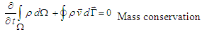
In this section, the mathematical formulation of governing equations for an inviscid compressible flow (Euler equations) in all flow regimes is to be discussed. For a passing flow in a volume Ω limited to the area of Γ, Euler equations are written as Eqs.(1),(2),(3).

(1)

Momentum conservation:

(2)

Energy conservation:

(3)

In the above equations, is density, is the velocity vector, p is pressure, is external forces, E is internal energy, and H is the total enthalpy of the fluid that can be written as. Eq.(4).

(4)

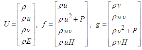
Total internal energy E is defined as and in this equation e is defined as which is the specific heat at constant volume. Above equations can be defined in a general and vector form. Hereby, if U is considered as the conservative variable tensor, is considered as flux vector, and is considered as unit matrix, it can be written as. Eq.(5).

, ,

(5)

If this equation is written in the differential and vector form, so we have. Eq.(6) as following:

(6)

In the 2D unsteady flow, the Cartesian components of U vector and F vector are described as. Eq.(7).

(7)

Where, u and v are the velocity components of . Thus, equation (6) can be written in the Cartesian coordinate as. Eq.(8).

(8)

Above equation is called Euler equation.

3. Calculation of Flux in an Oblique Surface

Noticing to the applied problems, the computational cells are not always diagonal and the cells’ lines are not in the flow direction; therefore, the passing flux can have both x and y components in the surface of cell. Thus, the equations and procedure of flux calculation should be changed. In the most previous works done by A. Harten, H.C. Yee and other researchers, the matrix of left and right agent vectors and other flux parameters were separately used in x and y directions. Finally, conversion from location coordinate to main coordinate is imposed to them after the calculations. But now, because cells and governing equations are discretized based on the finite volume and the computational cell is the same physical cell, the method that be used for calculation of flux is based on the Hirch method (1990) in the way that all terms of flux and its elements in the location direction of =(x,y) and =(x,y) are decomposed to the x and y directions, and then are added together. Thus, it is necessary to investigate the cell geometry and position of cell surface relative to the center of surrounding cells. Geometry used in calculating the flux is shown in fig.1.

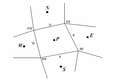Figure 1. Geometry used in calculating the flux

3.1. Calculation of Flux at e Surface

In order to calculate the passing flux in the e surface of cell, the surface shown in the figure 1 is considered. If this surface is separately to be investigated, an arbitrary position of that surface in the locational coordinate (ξ,η) is related to the main coordinate (x,y) as figure 2.

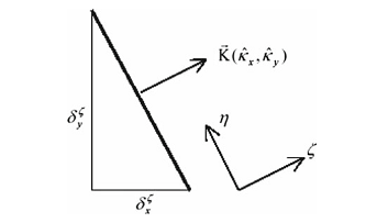Figure 2. Cell surface e in the local coordinates

The geometrical equations for above case can be written as equation 9.

(9)

So, according to the symbols of figure 1, can be written as equation 10:

(10)

As it can be seen, and are the Cartesian components of unit vector of . This unit vector is perpendicular to the surface of cell, and put along the locational direction. Noticing to the above equations, flux of velocity vector in direction can be defined as Eq.(11).

(11)

The conservative vector of variables is shown by U, conservative vector of mass flux, momentum and energy in each centers of surrounding cells of e surface areas. Eq.(12).

(12)

For an arbitrary cell, flux at the e surface is determined as. Eq.(13).

(13)

In this equation, are the agent values and show the characteristic variables. In the hyperbolic equations system, four agent values at the mentioned surface for a 2D flow areas. Eq.(14).

(14)

The characteristic values of α at the e surface are computed by multiplying each row of left agent matrix to the conservative variables as. Eq.(15).

(15)

Above equations in the general and vector form are defined as. Eq. (16).

(16)

L and R are the center of left and right cells of e surface respectively. is the i^th row of the left agent matrix and ~ shows that matrix is defined at the surface of e cell and its components are based on the Roe averaging method. r_i in .Eq.(13) is the i^th column of matrix which is described as. Eq.(17).

(17)

Based on the second order upwind TVD approximation, Yee et al. supposed the equation.(18) for displacement discretization of diffusion term.

(18)

Where the function of γ is as Eq.(19).

(19)

In above equations, is the characteristic value of l^th characteristic at the surface of e cell, is the limited function related to the l^th characteristic at the center of i^th cell, is the characteristic variable at the surface of e cell which is equaled to l^th column of matrix, and finally is the enthalpy function. Harten and Hyman suggested above assumption as .Eq.(20)

(20)

In this equation, is zero for flow containing dynamic shock waves and have a small value for static shock waves. Various functions are to be considered for limited function at the center of cell. Yee et al. suggested many of these function that in the present study, one of them is used as. Eq.(21).

(21)

In order to avoid any problem in computations, Yee et al. introduced the equations 22 for enthalpy and gamma functions, and , in all computations.

(22)

4. Reduction of TVD Error Using Artificial Compression Method (ACM)

As it was explained, when discontinuities is occurred, high resolution method such as TVD and ENO prevent to create oscillations by decrement of order while the diffusion is increased. Hereby, the accuracy of shock waves capturing is decreased in the discontinuities; therefore, finding a method for modifying this phenomenon is essential. Harten introduced a new method for increasing the accuracy of first order scheme in the shock wave capturing of discontinuities zones. Yee et al. used above method for viscous flow as. Eq.(23).

(23)

In this equation, the diffusion function is combined by TVD and anti-diffusion functions (Harten switch) in which the anti-diffusion function is directly imposed to it.

(24)

(25)

In this equation, is the anti-diffusion function at the surface of i^th cell related to the l characteristic and k is a variable that depends on the properties of problem. In this study, in order to increase the accuracy and decrement of diffusion in discontinuities, another approach is considered for imposing the ACM to diffusion term of TVD. With noticing to the previous points, ACM cannot be imposed to diffusion term directly, therefore, the anti-diffusion function is imposed to the limited function, which is put into the diffusion term and affects on it. The used method is as. Eq.(26).

(26)

As it can be seen, the g function is replaced by the generated limited function in the diffusion term of TVD. is the coefficient of ACM in this equation. Because each wave (linear and nonlinear wave) has a particular diffusion, we have different coefficients relative to the other characteristics for each characteristic. is defined as equation 27 in i^th cell for each characteristic of l.

(27)

α is the characteristic variable computed at the surface of cell. is a coefficient that is different for various characteristics and is function of flow physics. Thus, it’s calculated by try-error method for a specific flow.

Based on the mentioned equations, the new limited function is greater than the limited function of TVD method. As a result, accuracy and convergence of solution are improved, which affect on improvement of the shock wave capturing. But, with increment of and consequently the limited function, the diffusion is too decreased and the convergence procedure is probably interrupted. Thus, should be defined in a specific range or should be have an optimum value for a specified flow, which in that values, increment of the accuracy doesn’t happen with more convergence reduction and computation time increment, which is discussed in the next section.

5. Results and Discussion

This section discusses about the outlet results from the solution of inviscid flows by Jameson, TVD, and ACM methods and compares them together. It’s also explained about the effect of numerical diffusion reduction on the results. The present topic is a 2D steady flow over a circular bump for a supersonic flow with Mach=1.4, 1.65 which is a suitable experiment in the computational fluid dynamic (CFD) for compressible flows computations.

Steady flow over a bump channel

The results are demonstrated for two inlet Mach numbers (1.4,1.65) and the thickness of the circular arc “bump” on the upper wall is 4% of the bump length. In Figure 3 the geometry of a 4% thick bump on a channel wall is shown together with the algebraic mesh (90×30) used to compute steady two-dimensional flow.

Also, figure 4 shows Mach distribution on the top wall, and figure 5 shows the Mach distribution on the bottom walls. Figure 6 and 7 indicate the pressure distribution on the top and bottom walls for all three methods respectively.

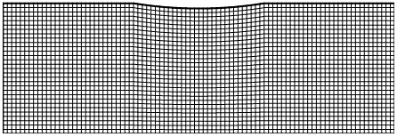Figure 3. Supersonic flow over 4% thick bump, inlet M=1.4 Supersonic bump geometry and 90*30 mesh

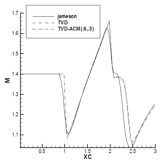Figure 4. Mach number on the upper wall inlet M=1.4

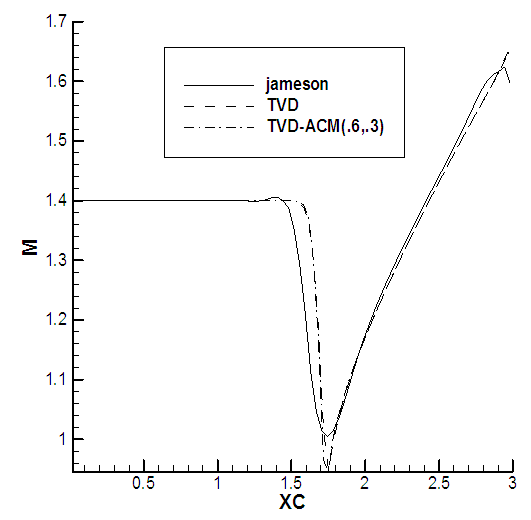Figure 5. Mach number on the lower wall inlet M=1.4

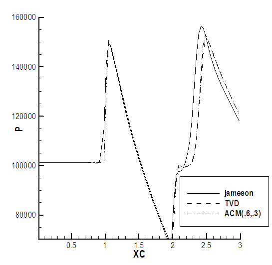Figure 6. Pressure on the upper wall inlet M=1.4

Figure 7. Pressure on the lower wall inlet M=1.4

5.1. Supersonic Flow with Mach 1.4

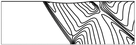
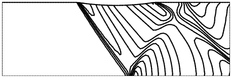
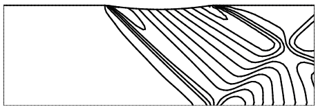
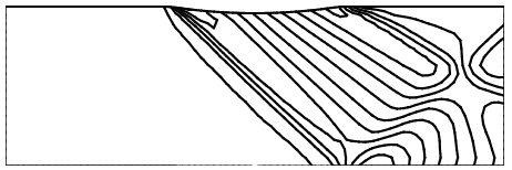
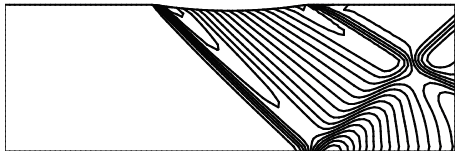
In this section, the supersonic, steady, and inviscid flow over a bump with the thickness of 4% is presented. The channel dimensions are standard and the inlet Mach is 1.4, and the general parameters are:

The length of computational meshing: 3m

Number of nodes (30 nodes in the y direction and 90 nodes in x direction).

Bump location: between the north boundary.

The computational meshing is shown in the figure 3.

According to the above diagrams, decrement of diffusion increased the accuracy in computation of Mach number and pressure in where the reflection of waves is happen. The contours of Mach are indicated in the figures 8,9,10 for showing the increment of the solution accuracy in whole computation domain.

The pressure contours for all three methods are indicated in the figures 11, 12, 13.

Figure 8. Mach contours (Jameson) inlet M=1.4

Figure 9. Mach contours (TVD) inlet M=1.4

Figure 10. Mach contours (TVD-ACM) inlet M=1.4

Figure 11. Pressure contours (Jameson) inlet M=1.4

Figure 12. Pressure contours (TVD) inlet M=1.4

Figure 13. Pressure contours (TVD-ACM) inlet M=1.4

As it observed, in the ACM method, all waves including shock waves propagation, waves interaction, and waves reflection from walls are better captured relative to the TVD and Jameson methods, which is shown the innovation and accuracy of the used method. Comparing the above figures illustrates the effectiveness of ACM method and its performance at the discontinuities. For TVD and Jameson methods, Mach contours are dispersed at the shock wave location due to the high values of numerical diffusion. On the other hand, in the ACM method, dispersion in capturing of the waves is decreased and the shock wave is better captured because of decreasing in the numerical diffusion. It’s noticeable that all physical and computational conditions are similar, and imposing the coefficients and anti-diffusion function to the limited function in the ACM method are only different.

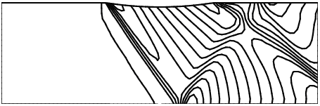
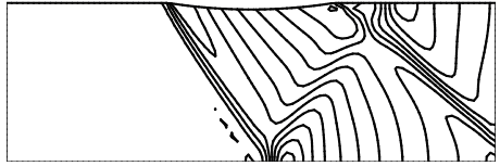
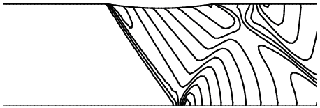
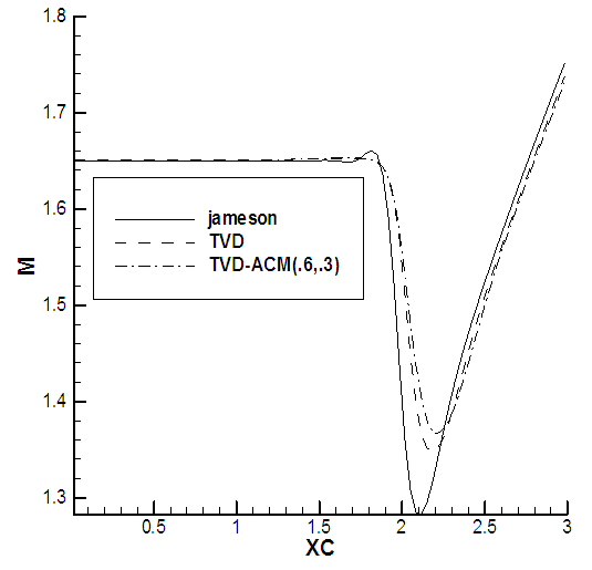
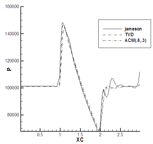
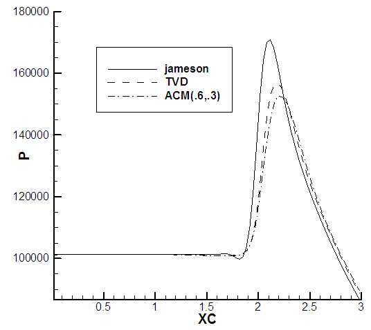
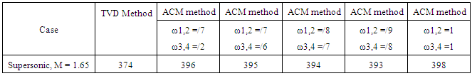
5.2. Supersonic Flow with Mach 1.65

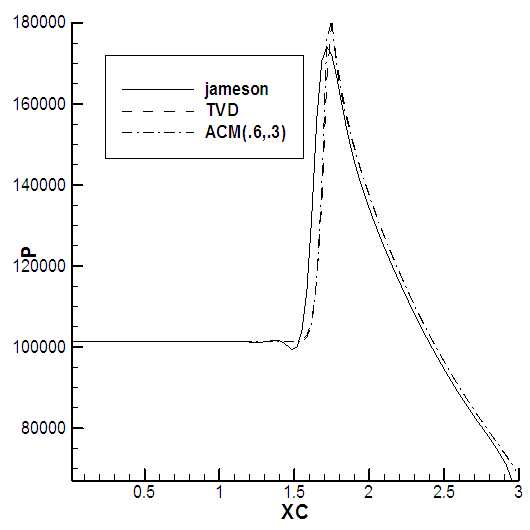
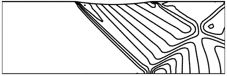
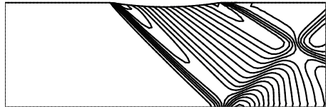
The dimension of the channel, kind and number of grids are similar to the previous case as shown in the figure 3. Only the inlet Mach number is different.

Figures 14 and 15 show the Mach distribution, and figures 16 and 17 indicate the pressure distribution on the top and bottom boundaries of the channel. Figures 18, 19, and 20 show the contour of Mach number inside the channel, and figures 21 to 23 show the pressure contour for all three methods.

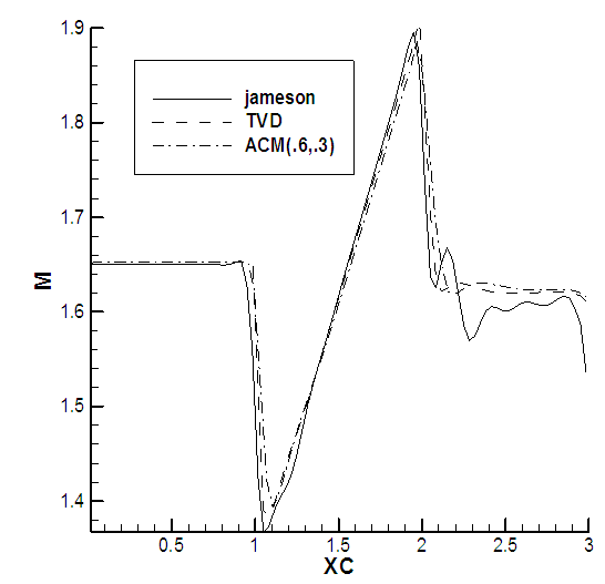Figure 14. Mach number on the upper wall inlet M=1.65

Figure 15. Mach number on the lower wall inlet M=1.65

Figure 16. Pressure on the upper wall inlet M=1.65

Figure 17. Pressure on the lower wall inlet M=1.65

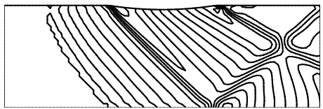Figure 18. Mach contours (Jameson) inlet M=1.65

Figure 19. Mach contours (TVD) inlet M=1.65

Figure 20. Mach contours (TVD-ACM) inlet M=1.65

Figure 21. Pressure contours (Jameson) inlet M=1.65

Figure 22. Pressure contours (TVD) inlet M=1.65

Figure 23. Pressure contours (TVD-ACM) inlet M=1.65

Although the density based algorithm is suitable for compressible flows, figure 18 don’t show a convenient capturing of the shock wave. Refraction is observed at the outlet due to the poor boundary condition or its lower order, while all waves including propagation of shock waves, interaction between waves, and reflection from walls are better captured at the outlet for TVD and ACM methods. It is also observed that the capturing of the reflected shock wave from upper wall and the outlet waves is improved by imposing the diffusion function to the ACM method.

6. Comparing of Solution Convergence and Computations Time for TVD, Jameson, and ACM Method

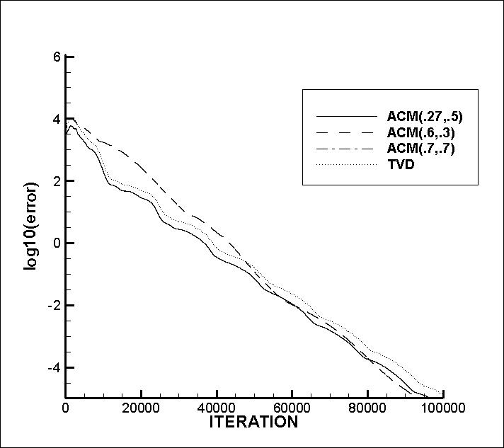
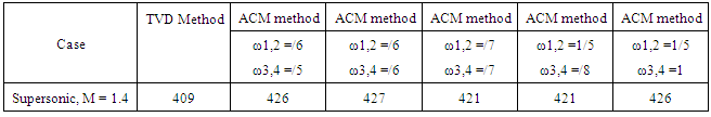
This section investigates solution convergence and computations time related to the numerical experiment of supersonic flow over the bump for each specific flow. Boundary condition and cell size are similar in calculation of different flow variables, and only difference is in imposing of the anti-diffusion function with various coefficients for ACM method. The residual history of velocity for supersonic case is shown in figure 24.

As it can be observed in figure 24, because of more operations and reduction of numerical diffusion of the ACM method in this flow, the solution convergence is achieved in more iterations for a specific accuracy relative to the TVD method. Note that, the first and second values in the parenthesis are related to the anti diffusion function for linear and nonlinear flow field in the ACM method.

Figure 25 shows the convergence diagram for supersonic flow with M=1.4 at the inlet. With noticing to this diagram, it can be indicated that the convergence of TVD method remains at the constant level after a specific iteration, and becomes horizontal, but when the anti-diffusion function is imposed in the ACM method, the convergence becomes better, and solution procedure is converged in lower accuracy. The effect of ACM coefficients is important in solution convergence that is shown in figure 26.

Thereby, convergence is improved with considering ω=0.27 and 0.5 for linear and nonlinear fields. As a result, quality of capturing is increased and diffusion in capture of discontinuities is decreased with increment of ACM coefficients. But, it’s difficult to conclude that the convergence is improved, because more decrement of numerical diffusion have a remarkable negative effect on the solution convergence. Thus, it’s necessary to find the optimum coefficients of anti-diffusion function in each flow. Residual history of velocity "u" for M=1.65 is shown in figure 27.

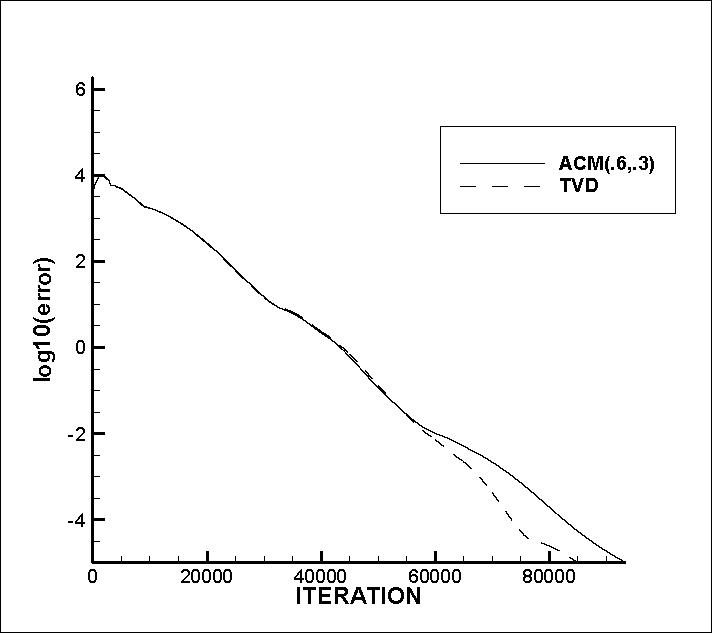Figure 24. Residual history of velocity "u" for supersonic case. The numbers in parenthesis (.6,.3) correspond to(ω1,2 ,ω3,4) for ACM, where ω1 and ω2 are considered for linear and ω3 and ω4 for nonlinear scopes

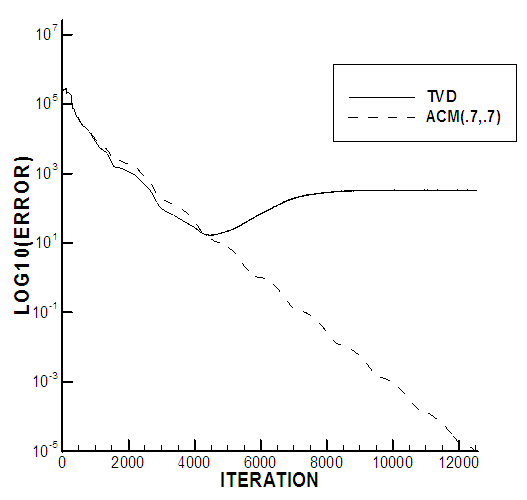Figure 25. Residual history of velocity "u" for M=1.4. The numbers in parenthesis (.7,.7) correspond to (ω1,2,ω3,4) for ACM, where ω1 and ω2 are considered for linear and ω3 and ω4 for nonlinear scopes

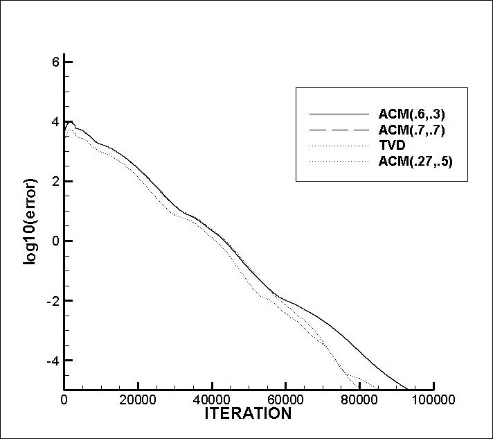Figure 26. Residual history of velocity "u" for M=1.4. The numbers in parenthesis (.7,.7) and (.27,.5) and (.6,.3)correspond to (ω1,2,ω3,4) for ACM , where ω1 and ω2 are considered for linear and ω3 and ω4 for nonlinear scopes

Figure 27. Residual history of velocity "u" for M=1.65. The numbers in parenthesis (.7,.7) and (.27,.5) and (.6,.3) correspond to (ω1,2,ω3,4) for ACM , where ω1 and ω2 are considered for linear and ω3 and ω4 for nonlinear scopes

As it is observed in figure 27, convergence is achieved in less iteration for lower residual target with imposing the anti-diffusion function to the ACM coefficients computations. Figure 28 shows the convergence diagram for M=1.65 at inlet for the bump channel. According to the figure 28, convergence improvement is significant for this flow in the way that in ACM coefficients of 0.9 and .5, the number of iteration is reduced about one per fifth for a specific residual target relative to the TVD method.

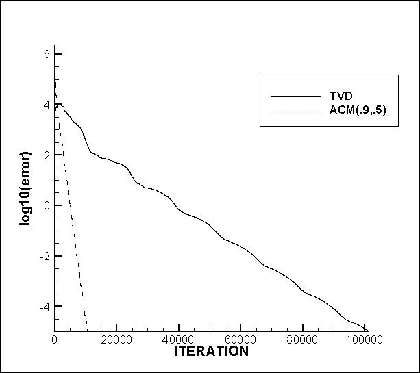Figure 28. Residual history of velocity "u" for M=1.65.The numbers in parenthesis (.9,.5) correspond to(ω1,2,ω3,4) for ACM, where ω1 and ω2 are considered for linear and ω3 and ω4 for nonlinear scopes

In order to investigate the effect of number of grids on the optimum coefficients of ACM, the flow with M=1.65 in the bump channel is chosen. The convergence diagram is shown in the figure 29. In this diagram, all conditions are similar except the grids.

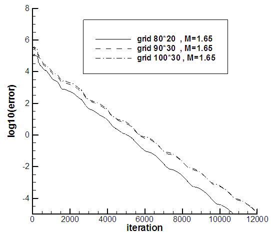Figure 29. Residual history of velocity "u" for M=1.65 for different the number of grid points. And the impact of the number of grid points on the optimal values of ACM coefficients

As it is obvious in the above diagram, solution is not converged in acceptable accuracies for coarse grid. On the other hand, the solution convergence is improved by decrement of ACM coefficients for nonlinear fields.

In this paper, it is need to investigate the time of computations for a specified accuracy or iteration. These results are tabulated in which the time of computations with various coefficients of ACM method are compared with TVD method vs. second. In the table 1 and 2 related to the supersonic flow over the bump channel, a specified iteration is the criterion; therefore, increment of running time in the ACM method should not be considered for achieving a specific accuracy, but also it’s interpreted as the time of operations.

According to the results of the table 1 and 2 at the equivalent iteration, running time is increased 5% for ACM method. On the other hand, it’s concluded that for an arbitrary accuracy (figure 27), convergence of ACM method is achieved faster than TVD method. Also, in order to avoid instability in solution convergence, optimum values of anti-diffusion coefficients of nonlinear fields should be less than linear fields.

Table 1. CPU time (s) for supersonic case until 3,000 iterations

Table 2. CPU time (s) for supersonic case until 3,000 iterations

7. Conclusions

In brief, the results of solving an incompressible flow with imposing the TVD, ACM, and Jameson methods to a density based algorithm are

1. By imposing ACM and TVD methods, limitation of density based algorithm in accuracy of particle waves capturing is somewhat improved in the compressible regime.

2. The characteristics velocities are better converged due to the augmentation of limiter, therefore, for a similar algorithm, ACM and TVD methods capture the shock waves with higher resolution relative to the Jameson method. Shock waves include simple waves, reflected waves, and waves interaction.

3. TVD method have a good quality in shock wave capturing in comparison to the published results of density based method, while have a less accuracy relative to the ACM method.

4. In this work, not only quality of capturing is improved for all flows at the discontinuities by ACM and TVD methods, but also the time of computations and convergence are improved for supersonic flows.

5. In order to stabilize the solution convergence and improve the solution procedure for coarse grids, the ACM coefficients should be less for nonlinear fields relative to the linear fields. Hereby, sufficient numerical diffusion is provided for stability of solution. On the other hand, reduction of computational cells decreases the operations, and consequently the convergence is improved.

6. Convergence improvement should be considered in various aspects of this paper including calculation and decomposition agent vectors, agent values, and passing flux over oblique surfaces into the main coordinate.

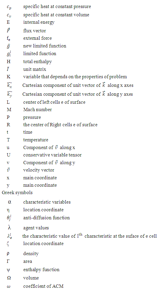
8. Nomenclature