1. Introduction

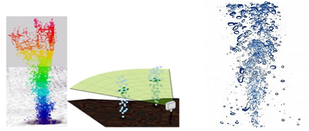
Multiphase flows encompass wide-ranging scales and a variety of phenomena. Multiphase flows are involved in solving many engineering problems. Approaches from a variety of points of view are actively being pursued to move this field forward. By getting a good understanding of verifying and skillfully using data that is captured, we can expect powerful designs and rationalized support techniques for many engineering applications (Naoki et.al. 2012).

The techniques of gas injection have been widely utilized in many engineering fields as materials, chemical, mechanical, and environmental engineering for improving chemical reactions, waste treatment, gas mixing and resolution, heat and mass transfer, and so on. Many researchers have carried out extensive model experiments by focusing on flow fields using air bubbles, because gas injection through a bottom nozzle is very popular and has wide applications. Bubble plume (Buoyant plumes produced by a source of bubbles in a liquid medium) which is a typical form of bubble flow, has received considerable attention in the last four decades and becomes a very important topic of research recently due to its large and wide range of applications value, and its effect on many processes and the efficiency of many devices. The motivation for studying bubble plumes is evident, from the fact that these plumes are encountered in a variety of engineering problems. In the past 10 years, the range of its application prompted scholars to do experiments and numerical research about this phenomenon. The bubble plume is known as one of the transport phenomena able to drive a large-scale convection due to the buoyancy of the bubbles. The flow in the vicinity of a free surface induced by a bubble plume is utilized as an effective ways to control surface floating substances on lakes, oceans, as well as in various kinds of reactors and industrial processes handling a free surface. The surface flows generated by bubble plumes are considered key phenomena in many kinds of processes in modern industries. Bubble plumes are observed in various engineering disciplines and fields, e.g. in industrial, materials, chemical, mechanical, civil, and environmental engineering applications such as chemical plants, nuclear power plants, naval engineering, the accumulation of surface slag in metal refining processes, the reduction of surfactants in chemical reactive processes, chemical reactions, waste treatment, gas mixing and resolution, heat and mass transfer, aeronautical and astronautical systems, biochemical reactors as well as distillation plants, etc. (Hassan 2002, 2003, 2006, 2011, 2012, 2013, Hassan and Tamer 2006, Abdulmouti, et. al. 2000, Hassan et. al. 1997, 1998, 1999- No. 1, 1999- No. 2 and 2001, Hassan and Esam 2013, Murai et. al. 2001, Abdel Aal et. al. 1966, Goosens and Smith 1975, Al Tawell and Landau 1977, Chesters et. al. 1980, Bankovic et. al. 1984, Sun and Faeth 1986a, b, Szekely et. al. 1988, Gross and Kuhlman 1992, Bulson 1968, and A.W.G. de Vries 2001).

Buoyant plumes driven by a source of gas bubbles have had a number of applications. They have been used with varying degrees of success. For instance, the following systems using bubble plumes were discussed in several literatures. (Taylor 1955) explained how bubble-breakwaters were operated by means of a surface jet produced by a bubble plume. He also demonstrated theoretically that the surface flow in the direction against the waves can break them. (Baines 1961) mentioned that the prevention of clean surface rivers or lakes from freezing over is possible using a bubble plume. (Baines and Leitch 1992) found that lines of bubble plumes have been used successfully to inhibit surface ice formation by bringing bottom water to the surface. They explained also that the most extensive application at that time was the destratification of reservoirs by mixing the lower-level water with the surface water. Denser water is lifted upward where the turbulence generated by the bubbles produces mixing with the lighter water. There is a similar process in metallurgical furnaces where the liquid metal or slag is heated from the top and hence is stratified. (Jones 1972) explained that bubble plumes can also contain oil slicks on water surfaces, and protect from underwater-explosion damage. (Marks and Cargo 1974) mentioned that bubble plumes were also useful for keeping swimming areas free from slow-moving objects such as sea nettles. Oil is very harmful to marine life and it is very difficult to clean the ocean from it (Hoults 1969). In addition, during an underwater oil-well blow-out, a plume of bubbles, oil droplets and sea water develops; the extent of the damage to marine life depends on whether all the oil rises to the surface or spreads out horizontally at some intermediate depth. Hence, another interest in bubble plumes arises in the context of rectifying an oil-well blowout. Characteristically a lot of gas is emitted with the oil, and a plume develops due to the presence of bubbles formed by this gas (Topham 1974). (Mcdougall 1978) explained that the extent of damage caused by an oil-well blowout was strongly dependent on whether all the oil rises straight to the surface or some of it spreads out horizontally at some intermediate depth. (Kobus 1968 and McDougall 1978) made analytical studies on the vertical rising flow using experimental constants. (Shoichi et al 1982) measured two dimensional surface flow velocity profiles using hot wires as a basic tool for studying the prevention of oil diffusion with the help of a bubble plume.

Furthermore, the bubble plume has been a key issue in the current research field of fluid mechanics. Bubble plumes have great application value in projects, such as alleviating the damage of wave to building structure, preventing the invasion of brine with air bubble curtain in estuary, controlling the stratification structure of reservoirs and lakes to improve water quality, preventing channel and harbor from being freezed, enhancing oxygen for aquatic growth and so on. Most especially in recent years, with the large-scale exploitation of oil and gas under the sea, the oil-gas blowout causes serious pollution to the sea, and bubble plumes can used to control the pollution area. Above all has greatly simulated the research on bubble plume to widen its applied range. Moreover, bubble plumes have received considerable attention in the last four decades due to its large range of applications. For example, they have been proposed as a means of containing surface-floating substances, such as oil from large oil spills in rivers and estuaries; they have been employed to augment convective heat and mass transfer rates in various chemical applications; they have been used as pneumatic breakwaters; they have been employed for preventing icing in navigational waterways. One area of application that has received a great deal of recent attention is the use of bubble plumes as a desertification device, inducing mixing while introducing dissolved oxygen for improving water quality in lakes and reservoirs (Cheng Wen et al. 2008, Hassan 2002, 2003, 2006, 2011, 2012, 2013, Hassan and Tamer 2006, Abdulmouti, et. al. 2000, Hassan et. al. 1997, 1998, 1999- No. 1, 1999- No. 2 and 2001, Hassan and Esam 2013 and Schladow 1992).

In addition, one of the reasons for the study of bubbly flows is their wide applications ranging from hydraulic engineering to high energy physics experiments. In particular, researcher interested in a recent application of bubbly fluids in the mitigation of cavitation damages in the Spallation Neutron Source (SNS) (Riemer et al. 2002). Another important motivation is to connect the microscopic behavior of individual bubbles to the macroscopic behavior of the mixed medium that one directly observes.

In industry, bubble plumes are used with two objectives: enhancing mass transfer and mixing. As a mixing technique, the use of bubbles is attractive because it is very simple and cheap to operate. The most common applications of bubble-driven mixing are encountered in wastewater treatment, in the delicate mixing of pharmaceutical and food products, in the mixing of very hot or toxic liquids and in the desertification of lakes and reservoirs.

Whereas, bubbly flows are central to many industrial processes. Heat transfer through boiling is the preferred mode in most power plants and bubble-driven circulation systems are used in metal processing operations such as steel making, ladle metallurgy, and the secondary refining of aluminium and copper. Similarly, many natural processes involve bubbles. Bubbles play a major role in the interactions of the oceans with the atmosphere, for example, and both air bubbles near a free surface and cavitation bubbles are of major importance for detection of submarines in naval applications (Asghar and Gretar 1998).

Moreover, flows induced by a bubble plume are utilized in many industrial processes. The main features of this kind of flow are:

(a) A large scale circulation of the liquid phase can be generated in natural circulation systems like lakes, agitation tanks, etc.

(b) Strong rising flows can be induced by the pumping effect as in air-lifting pumps.

(c) High speed surface flows may be developed at the free surface, by which the density and the transportation of the surface floating substances can be controlled.

(d) A high turbulence energies can be produced in the two-phase region due to the strong local interaction between individual bubbles and the surrounding liquid flow. (Hassan 2002, 2003, 2006, 2011, 2012, 2013, Hassan and Tamer 2006, Abdulmouti, et. al. 2000, Hassan et. al. 1997, 1998, 1999- No. 1, 1999- No. 2 and 2001, Hassan and Esam 2013, Murai et. al. 1999, Murai et. al. 2001).

Hence, by applying the bubble plume, the following processes are expected to be improved:

1- The prevention of sea water pollution by heavy oil leakage from tankers. Moreover, the development of the technology to prevent the diffusion of the leaked oil or oil generated from oil sources in the sea.

2- The prevention of diffusion of organic or harmful substances on the sea surface, lake surfaces and river surfaces, and the forced collection of them using the surface flow.

3- The prevention of freezing over of the surfaces of seas and lakes in winter season.

4- Damping of waves propagating on the sea, lakes and rivers.

5- Accumulation of the surface slag in the metal refining process.

6- The reduction of surfactants in chemical reaction processes. Beyond that, removal of oxide films or floating impurities from the surface of the chemical reactors in order to maintain the performance of reactions.

7- Prevention of surface sloshing in furnaces. Beyond that, removal of oxide films or floating impurities from the surface of the metal refining furnaces in order to maintain their performance. (Hassan 2002, 2003, 2006, 2011, 2012, 2013, Hassan and Tamer 2006, Abdulmouti, et. al. 2000, Hassan et. al. 1997, 1998, 1999- No. 1, 1999- No. 2 and 2001, Hassan and Esam 2013).

Bubble plume, which is a special case of bubbly flow, has become a very important topic of research recently due to it wide applications, and its effect on many processes and the efficiency of many devices. In the past 10 years, the range of its application prompted scholars to do experiments about this phenomenon. Most of these experiments were focusing on determining time-averaged velocities in small and big tanks. Some scaling relations were proposed to the bubble plume available applications. The focus was on vertical direction in vassals and later on including the radial or the horizontal one. Also, the procedure to analyze how to plumes interact, and the velocity distribution and turbulence aspect in tanks were attractive and interested points to be studied.

On the other hand, bubbly flows are encountered in many fields of engineering, pertaining to different spatial scales. At the small scale, they are found for instance in metallurgy in gas stirring of ladles, in nuclear devices, and chemical reactors; at extremely large scale, they take place in induced events of carbon dioxide sequestration, by which this compound is “injected” into deep seas. At the environmental scale, the application range is vast: bubble plumes have been used as barriers to contain density intrusions or oil spills, as breakwaters, as silt curtains, and in lakes for destratification purposes. In sanitary engineering, bubble plumes are usually employed for aeration purposes in water and wastewater treatment plants. Additionally, arrays of bubble diffusers are used in reservoirs aimed at storing combined sewer overflows, in order to avoid the occurrence of anaerobic conditions (Fabian 2004).

Beyond that, air-bubble systems have been used extensively and for a variety of purposes such as, pneumatic breakwaters, prevention of ice formation, as barriers against salt water intrusion in rivers and locks, for stopping the spreading of oil spills on the water surface, for reduction of underwater explosion waves and for agitation and mixing operations in process industries. However, the technique may also be used for destratification and water quality control management of lakes and, reservoirs in which case the characteristics of the air-bubble plume are of more interest than the induced horizontal flow in the surface layer (Klas and John 1970).

Whereas, the motivation for studying bubble plumes is evident, from the fact that these plumes are encountered in a variety of engineering problems. To mention a few, plumes have been used to damp sea waves in harbors (pneumatic breakwaters), to prevent surface ice formation in harbors, to mix stratified fluid layers, to re-aerate lakes, and to protect installations from shock waves produced by underwater explosions (cf., for instance, Kristian and Iver 2008).

With increasing subsea activities plumes have acquired increased importance from a risk assessment point of view. It becomes imperative to obtain knowledge about the implications of a rupture, or even a breakage, of a subsea pipeline. Thus in case of an underwater blowout of inflammable gas, the following points are very important in studding the plumes:

• The concentration of gas at the free surface.

• The extension of the area covered by gas at the free surface.

• The rising time of the gas. (Kristian and Iver 2008, Hassan 2002, 2003, 2006, 2011, 2012, 2013, Hassan and Tamer 2006, Abdulmouti, et. al. 2000, Hassan et. al. 1997, 1998, 1999- No. 1, 1999- No. 2 and 2001, Hassan and Esam 2013).

In addition, a two-phase flow is one of the most common flows in nature as well as in many applications especially industrial; it covers gas-solid, liquid-liquid, solid-liquid and gas-liquid flows. Among these, the gas-liquid flows can be encountered in wide variety of industrial applications including boilers, distillation towers, chemical reactors, oil pipelines, nuclear reactors, etc. The measurement of two-phase flow parameters such as flow regime, bubble size and shape, bubble velocity and void fraction is considerably important and plays an important role in operational safety, process control and reliability of continuum processes (Dong, F. et al., 2003, Hassan 2002, 2003, 2006, 2011, 2012, 2013, Hassan and Tamer 2006, Abdulmouti, et. al. 2000, Hassan et. al. 1997, 1998, 1999- No. 1, 1999- No. 2 and 2001, Hassan and Esam 2013).

As a summary, it is clear that the bubble plume “which is a typical bubble flow” is a key phenomenon to be studied and investigated, and it is an effective tool for many applications and can indeed contribute to various improvements. The motivation to study the bubble plume is the demands to improve its performance and its applications. Especially in many engineering fields as materials, chemical, mechanical, modern industrial technologies, and in the environment in order to protect the natural environment, the naval planets, navel systems, rivers, lakes, etc., from pollution. Hence, these engineering fields are expected to benefit from the improvement and development of the bubble plume.

The motivation of the present work which is part-I is the dement to demonstrate, review and summarize the major finding of previous research of bubbly two-phase flow characteristics, behaviors and flow patterns. Furthermore, to elucidate some techniques and the important models for the measurement of the dominated two-phase bubbly flow/ bubble plume parameters such as flow regime, bubble size and shape, bubble velocity and void fraction which are considerably important and play an important role in operational safety, process control and reliability of continuum processes of many engineering applications.

In our paper (part-II), some others techniques and the important models for the measurement of the dominated two-phase bubbly flow/bubble plume parameters are elucidated, the turbulent bubbly flow structures are demonstrated. In addition, some other important applications especially on bubbly two-phase flow/bubble plume and its associated surface flow are presented.

2. Introduction to Multiphase Flow

The subject of multiphase flows encompasses a vast field, a host of different technological contexts, a wide spectrum of different scales, a broad range of engineering disciplines and a multitude of different analytical approaches.

The term multiphase flow is used to refer to any fluid flow consisting of more than one phase or component. Consequently, the flows have some level of phase or component separation at a scale well above the molecular level. This still leaves an enormous spectrum of different multiphase flows. One could classify them according to the state of the different phases or components and therefore refer to gas/solids flows, or liquid/solids flows or gas/particle flows or bubbly flows and so on; many texts exist that limit their attention in this way. Some treatises are defined in terms of a specific type of fluid flow and deal with low Reynolds number suspension flows, dusty gas dynamics and so on. Others focus attention on a specific application such as slurry flows, cavitating flows, aerosols, debris flows, fluidized beds and so on; again there are many such texts. The basic fluid mechanical phenomena were identified in order to illustrate those phenomena with examples from a broad range of applications and types of flow (Christopher 2005).

Parenthetically, it is valuable to reflect on the diverse and ubiquitous challenges of multiphase flow. Virtually every processing technology must deal with multiphase flow, from cavitating pumps and turbines to electrophotographic processes to papermaking to the pellet form of almost all raw plastics. The amount of granular material, coal, grain, ore, etc. that is transported every year is enormous and, at many stages, that material is required to flow. Clearly the ability to predict the fluid flow behavior of these processes is central to the efficiency and effectiveness of those processes. For example, the effective flow of toner is a major factor in the quality and speed of electrophotographic printers. Multiphase flows are also a ubiquitous feature of our environment whether one considers rain, snow, fog, avalanches, mud slides, sediment transport, debris flows, and countless other natural phenomena to say nothing of what happens beyond our planet. Very critical biological and medical flows are also multiphase, from blood flow to semen to the bends to lithotripsy to laser surgery cavitation and so on. No single list can adequately illustrate the diversity and ubiquity; consequently, any attempt at a comprehensive treatment of multiphase flows is flawed unless it focuses on common phenomenological themes and avoids the temptation to digress into lists of observations (Christopher 2005).

Two general topologies of multiphase flow can be usefully identified at the outset, namely disperse flows and separated flows. By disperse flows we mean those consisting of finite particles, drops or bubbles (the disperse phase) distributed in a connected volume of the continuous phase. On the other hand, separated flows consist of two or more continuous streams of different fluids separated by interfaces (Christopher 2005).

Two-phase flows with phase change occur in many engineering systems. Of specific interest are two applications involving wide range of length and time scales: (a) bubbly turbulent flows in the ship boundary layers for drag reduction and (b) hydrodynamics of cavitation. These problems share common physical mechanisms of mass, momentum, and energy exchange across the interface between the two phases (E. Shams et. al. 2010).

The dispersed bubbles may deform, vary in size, or coalesce and the local grid resolution may be such that the bubble is fully resolved or under-resolved in relation to the resolution of the background mesh as shown in Figure 1. In cavitating flows, the vapor cavity size can change dynamically and the local grid resolution may be such that the cavities (or bubbles) are fully (or partially) resolved on the grid or completely sub-grid. Different approaches are needed to model these flow regimes accurately (E. Shams et. al. 2010).

Figure 1. Schematic of fully resolved and subgrid disperse phase

Multiphase Flow Models

Multi-phase flows appear in numerous forms in Nature. They can be found in sediment-laden flows in rivers, in underflows associated with volcanic eruptions, in turbidity currents, in the bubbly wake of ships and in liquid-vapor mixtures in nuclear reactors, among many others. Basic aspects of the flow in a bubble plume were addressed by (Fabian et. al. 2004), which is a simple paradigm of multiphase flow that appears in a many situations: They can be used as breakwaters, as destratification devices, and as containment for oil spills; they are also encountered in oil-well blowouts and in nuclear devices.

Although multiphase flows have been very well-known for long time, the theory to explain them is still under development. Mass, momentum, and energy equations for each of the phases are nowadays available. These equations are much more complex than their single-phase counterparts and they pose new challenges to their analytical and numerical treatment.

Several numerical solutions of the two-phase flow equations have been presented in the last decade. Still, the prediction capability of the models is not fully satisfactory, with the exception of a few cases. The advancement of computational power has not provided means to compensate the inherent theoretical difficulties of multi-phase flows.

The modeling of bubble plumes has received attention in the engineering community with special emphasis in the analysis of the flow in reactors and in ladles. The results typically show an acceptable prediction of time-averaged variables, but the analysis of turbulence is far from being well established. Very often, the description of turbulence in bubble plumes determines the difference between having a physically correct result, exceeding the issue of accuracy of the solution (Fabian et. al. 2004).

A persistent theme throughout the study of multiphase flows is the need to model and predict the detailed behavior of those flows and the phenomena that they manifest. There are three ways in which such models are explored:

(1) experimentally, through laboratory-sized models equipped with appropriate instrumentation,

(2) theoretically, using mathematical equations and models for the flow,

and (3) computationally, using the power and size of modern computers to address the complexity of the flow. Clearly there are some applications in which full-scale laboratory models are possible. But, in many instances, the laboratory model must have a very different scale than the prototype and then a reliable theoretical or computational model is essential for confident extrapolation to the scale of the prototype. There are also cases in which a laboratory model is impossible for a wide variety of reasons (Christopher 2005).

Consequently, the predictive capability and physical understanding must rely heavily on theoretical and/or computational models and here the complexity of most multiphase flows presents a major hurdle. It may be possible at some distant time in the future to code the Navier-Stokes equations for each of the phases or components and to compute every detail of a multiphase flow, the motion of all the fluid around and inside every particle or drop, the position of every interface. Nevertheless, the computer power and speed required to do this is far beyond present capability for most of the flows that are commonly experienced. When one or both of the phases becomes turbulent (as often happens) the magnitude of the challenge becomes truly astronomical. Therefore, simplifications are essential in realistic models of most multiphase flows (Christopher 2005).

In disperse flows two types of models are prevalent, trajectory models and two-fluid models. In trajectory models, the motion of the disperse phase is assessed by following either the motion of the actual particles or the motion of larger, representative particles. The details of the flow around each of the particles are subsumed into assumed drag, lift and moment forces acting on and altering the trajectory of those particles. The thermal history of the particles can also be tracked if it is appropriate to do so. Trajectory models have been very useful in studies of the rheology of granular flows primarily because the effects of the interstitial fluid are small. In the alternative approach, two-fluid models, the disperse phase is treated as a second continuous phase intermingled and interacting with the continuous phase. Effective conservation equations (of mass, momentum and energy) are developed for the two fluid flows; these included interaction terms modeling the exchange of mass, momentum and energy between the two flows. These equations are then solved either theoretically or computationally. Thus, the two-fluid models neglect the discrete nature of the disperse phase and approximate its effects upon the continuous phase. Inherent in this approach, are averaging processes necessary to characterize the properties of the disperse phase; these involve significant difficulties. The boundary conditions appropriate in two-fluid models also pose difficult modeling issues (Christopher 2005).

In contrast, separated flows present many fewer issues. In theory, one must solve the single phase fluid flow equations in the two streams, coupling them through appropriate kinematic and dynamic conditions at the interface. Free streamline theory (see, for example, Birkhoff and Zarantonello 1957, Tulin 1964, Woods 1961, Wu 1972) is an example of a successful implementation of such a strategy though the interface conditions used in that context are particularly simple (Christopher 2005).

In addition, the simultaneous flows of more than one phase are almost ubiquitous particularly in the field of chemical engineering. These multiphase flows are complex because of the infinitely deformable nature of the interface in gas/liquid and liquid/liquid flows. It the case when one of the phases is a solid, dispersed phase, the complexity arises from the non-uniform distribution of particles about the pipe cross-section and axially. In order to handle these complexities, the different distributions of flows are usually gathered into groups called flow pattern. This approach is useful for modeling the flows. Methods for identifying the occurrence of particular flow patterns are provided together with models for pressure drop specific to those flow patterns. In addition, overall, more empirical methods are outlined. The information is presented for gas/liquid (including foams), liquid/liquid (including emulsions), gas/solid and liquid solid flows. Flow in pipes and in pipe fittings are examined as well as in the geometry usually termed bubble columns used in chemical reactors. Recent developments in modeling using advanced computational techniques are introduced (B.J. Azzopardi 2012).

Furthermore, multiphase flow, the simultaneous flow of more than one phase, occurs in many facets of chemical engineering, e.g., distillation, absorption, evaporation, condensation, solvent extraction. It is particularly prevalent and important in hydrocarbon production and refining, minerals transport, power generation as well as in many environmental applications. The possible combinations of phases are: gas/liquid; gas/solid; liquid/solid; the simultaneous flow of two immiscible liquids and gas/liquid/solids. The first four can be termed two-phase flow. The last, more complex case can be found in some catalytic reactors. Hydrocarbon production can involve the flow of gas, oil, water and solids emerging from the reservoir (B.J. Azzopardi 2012).

A complication of these flows is that the phases can be dispersed unevenly about the pipe cross-section and axially. This has important implications for the flow particularly the pressure drop/ flow rate/geometry relationships which are central to designers. It also has import for the separation of the phases. The phase disposition can be especially complex in the case of gas/liquid and liquid/liquid flows. The extremely deformable nature of the interface leads to a large number of possible configurations. Even with gas/solids and liquid/solid flows there can be systematic variations of the temporal and spatial concentration of the dispersed solids. It is because of these factors that workers in the field have used the concept of flow patterns-general descriptions of the disposition of the phases. Flow patterns, methods are outlined below, for gas/liquid (B.J. Azzopardi 2012).

Gas/Liquid Flows:

The particular complications of two-phase gas/liquid flows are caused by the interface between the phases as shown in the figure 2. This produces a wide range of configurations in the channel with consequences both for the hydrodynamics and for heat and mass transfer. The groupings of similar configurations are important as studies have shown that a single correlation for the whole range of gas/liquid flows from 100% liquid to 100% gas is inadequate. In addition, advanced codes for transient analysis use descriptions specific to individual flow patterns (or configurations) (B.J. Azzopardi 2012).

Figure 2. Samples of the two-phase gas/liquid flows

3. Bubble Behavior and Characteristics

The behavior of bubbles in a liquid is fundamentally different from that of solid particles in a gas. Bubbles have essentially no mass compared to the surrounding liquid, but particle inertia dominates the surrounding gas. Therefore, bubble motion leads the fluid while particles lag and the relative velocity is generally positive for bubbles but negative for particles. In fact, there is an interaction between the bubble plume and its environment. Hence, measurements of the environment can be used to derive the entrainment flux to the plume. Furthermore, an expression for the parameters is important in order to study the characteristic and the response of bubbles to the surrounding liquid (Hassan 2002, 2003, 2006, 2011, 2012, 2013, Hassan and Tamer 2006, Abdulmouti, et. al. 2000, Hassan et. al. 1997, 1998, 1999- No. 1, 1999- No. 2 and 2001, Hassan and Esam 2013).

As known, any substance with particles move easily among themselves is called fluid like gases and liquid. As a result, fluid can be either gas or liquid, in this case the fluid called single phase or a combination between these two-phases gas and liquid which called Two-Phases Fluid.

Bubble flow can also be named as bubble plume, plumes are interacting collections of bubbles formed by any action. For example, in seas plumes can be formed by natural source such as wave or submerged source like submarine.

Bubbly two-phase flows have various flow structures, which are not observed in a single-phase flow, due to the complexity of the translational motion and the volumetric change of the bubbles. The variety of the flow structure often considerably affects the performance of hydraulic machinery and chemical and bioreactors in which the bubbly media is used as a working fluid. Especially, the local flow behavior such as the mutual interaction between bubbles and vortices influences the statistical characteristics of the flow. For instance, both the generation and deformation of vortices in the liquid phase due to the inhomogeneous buoyancy caused by the local distribution of bubbles, and the accumulation of bubbles in the vortex cores and turbulence generation due to the bubble migration, enhance the flow instability and the turbulence modification. The bubble plume is a suitable object to analyze the detailed flow structure in bubble flow because it involves various interactions between the bubble and the ambient liquid flow when the bubble rises from the bottom to the upper free surface (Hassan 2002, 2003, 2006, 2011, 2012, 2013, Hassan and Tamer 2006, Abdulmouti, et. al. 2000, Hassan et. al. 1997, 1998, 1999- No. 1, 1999- No. 2 and 2001, Hassan and Esam 2013, Murai and Matsumoto 1998, Matsumoto and Prosperetti 1997, The Japanese Society of Nuclear Power Edit. 1992, Matsumoto and Murai 1995).

The bubble motion in a gas-liquid two-phase flow is one of the most important topics with respect to its irregular and complex flow features due to bubble deformation and density differences. One point measurement methods cannot obtain the unsteady features of the whole flow field including time-variations of the bubble motion. However, PIV is a powerful tool to investigate these features of the whole unsteady flow field. (Hassan 2002, 2003, 2006, 2011, 2012, 2013, Hassan and Tamer 2006, Abdulmouti, et. al. 2000, Hassan et. al. 1997, 1998, 1999- No. 1, 1999- No. 2 and 2001, Hassan and Esam 2013).

3.1. The Path of Free Rising Bubbles and Shape Instability

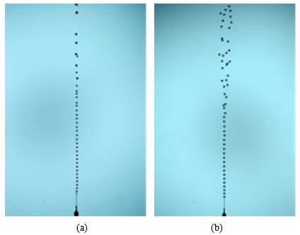
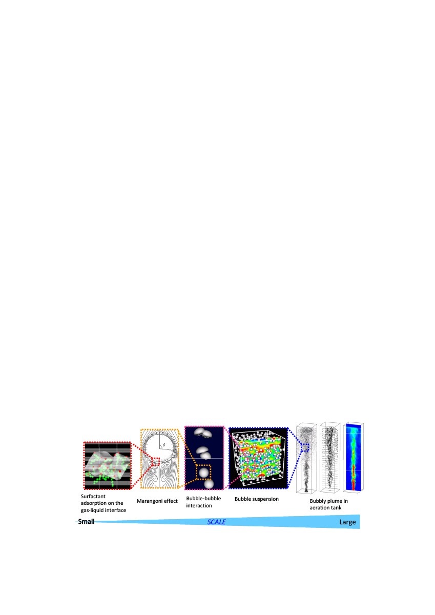
(Moore 1963, 1965) analyzed the effects of shape and boundary layer on the rise velocity of bubbles in a liquid of low viscosity. Many researchers have studied the path of free rising bubbles experimentally, (Maxworthy et al. 1996) performed the experiments in perfectly clean fluids. Consequently, (A.W.G. de Vries 2001) showed that the contamination of the fluids in most experiments is the reason for the differences in the parameters indicating the transition between the occurrence of straight-rising, spiralling and zigzagging path of bubbles. (A.W.G. de Vries 2001) simultaneously visualize, in a three dimensional way, the path and wake of a free rising air bubble in hyper clean water. The path of a rising bubble in hyper-clean water is correlated with the wake behind the bubble. A double-threaded wake occurs for bubbles moving in a non-rectilinear path. The non-rectilinear path, both spiralling and zigzagging, is in our view maintained by a lift force and not by vortex shedding, as is observed for solid spheres and for bubbles in contaminated water. The strength of this lift force is indirectly determined. For the zigzag, the lift force changes sign in the mean position of the zigzag. On the other hand, (Lunde and Perkins 1997) used a salted dye solution to conclude that vortex shedding is the mechanism for a bubble performing a zigzagging path in clean water. This conclusion is questionable with (A.W.G. de Vries 2001).

From all their experimental results and studies, the three observed paths are presented:

1) Straight rising.

2) Zigzagging.

3) Spiralling.

Based upon the experimental results a wake model is developed by (A.W.G. de Vries 2001) that explains the path of the bubble. In this model, a lift force is employed. The magnitude of this lift force is indirectly determined in several ways.

Experiments for bubbles with equivalent radii of 0.4-1.1 mm showed a clear transition from a rectilinear path to a zigzag or spiral path. This transition occurred for bubbles with equivalent radii of 0.81 mm or Reynolds number Re=740. After the transition, both zigzagging and spiralling bubbles were observed (cf. Saffman 1956). In (A.W.G. de Vries 2001) study, it was observed that the majority of the zigzagging bubbles were found to be of the size of 0.81-0.88 mm and 1.00-1.10 mm. The angular motion of the spiral has no preferred direction; clockwise or anticlockwise and the top view of the path is an ellipse and not necessarily a circle. A zigzag motion appears to be a special case of a spiral; one axis of the top view has zero length. Although a spiral and a zigzag path are fundamentally the same, both are separately mentioned to explain the differences in the development of the wake. For a rectilinear path, the wake consists of a single-threaded wake. After path instability sets in, a double-threaded wake is observed (Figure 3 and 4). The initial disturbance of the wake determines the rate of growth of the instabilities in the wake (A.W.G. de Vries 2001).

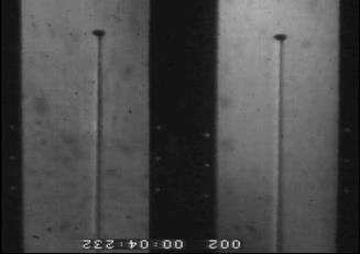Figure 3. The single-threaded wake behind a rectilinear rising bubble (req = 0.79 mm). On the left the XZ view and on the right the YZ view. The black areas are part of the reference system outside the water tank. The walls of the tank and the mirror inside the tank are over 20 bubble radii away from the bubble by view (A.W.G. de Vries 2001)

Figure 4. Different behavior of bubble chain at different Reynolds number (20 < Re < 100) (ultra-pure water) by (Petr et. al. 2007)

At low Reynolds numbers a bubble moves rectilinearly, while at higher Reynolds numbers oscillatory motions, as spiralling and zigzagging, are observed. Furthermore, the shape of the bubble is said to be stable for low Weber number and becomes oscillatory, or unstable, for larger Weber number (O (3)). The onset of path instability and that of shape instability are, in general, and also for bubbles in pure water, occurring at different stages (Saffman 1956, Hartunian and Sears 1957, Moore 1965 and Miksis et al. 1981).

Above a certain volume, bubbles rising in clean water perform unsteady irregular motions. For solid spheres a similar behavior is observed, although at lower Reynolds numbers (Re≈200) than for bubbles (Re≈600). The main differences between bubbles and solid spheres are the conditions at the boundary: no-slip and rigid for solids, zero-tangential-stress and deformable for bubbles. These differences influence the vorticity production at the surface and the drag. Contamination of the water may result in solid-sphere like behavior of the bubble.

3.1.1. Straight Rising Bubble

It is well known that a small bubble rises along a rectilinear path. In the experiments this occurs for equivalent radii less than about 0.81 mm, We_cr < 2.7 and Re <740, which is in agreement with the results of (Tsuge and Hibino 1977 and Benjamin 1987), taking into account the temperature effects (Morton dependence of critical Weber and Reynolds number). The schlieren visualization of a straight rising bubble is presented in Figure 3. It shows the three dimensional single-threaded wake behind the bubble in pure water. The three dimensions (3D) views were studied as 2 views, the first one located on the left side of the figure which is the XZ view where Z is the vertical direction and X is the horizontal direction. The second one is located on the right side of the figure that is the YZ view, where Z is the vertical direction while Y is the horizontal direction (A.W.G. de Vries 2001).

In Figure 3 the two perpendicular projections of the bubble and its wake are visible. It is obvious that this bubble is straight rising as in both views the path is straight. The black areas on the side of both projections belong to the reference system. The reference points are the lighter spots. The vertical distance between these points is 0.5 cm. It can be seen in Figure 3 that the reference points between the two perpendicular views are displaced vertically, which indicates that both views are not perfectly aligned. This misalignment is compensated for in the analysis. The reference system is placed outside the water tank and therefore will not influence the motion of the bubble. The walls of the water tank and the mirror placed inside the tank are over 50 bubble radii away from the bubble. Consequently, the motion is not influenced by wall effects (A.W.G. de Vries 2001).

Although it is not (clearly) visible in the images, there exists a vertical temperature gradient in the water column. The bubble drags some colder water in its wake. For reference purposes, denote the direction from left to right in both projections as positive. In a horizontal plane the temperature changes with position in both projections: i.e., from left to right, in the plane outside the wake warm, inside the wake colder and outside the wake again warmer. A negative temperature gradient in horizontal direction, or in other words a positive gradient in refractive index, is visualized with a positive gradient in the intensity (a lighter area). A positive gradient in the temperature results in a darker area. Consequently, the single-threaded wake is visible as a lighter and a darker streak. The relation between grey scale and temperature gradient is connected to the orientation of the schlieren gradient filter. The schlieren images clearly show the stable single-threaded wake (A.W.G. de Vries 2001).

In the vertical direction hardly any change in brightness is observed. This clearly indicates that the (A.W.G. de Vries 2001) schlieren setup is only visualizing the horizontal temperature gradient. It has to be noted, however, that in the vertical direction the measurement technique only detects the curvature of the temperature profile. This implies that the imposed temperature gradient is indeed constant.

Furthermore, it can be observed that the shape of the bubble is not spherical. In fact, it is nearly ellipsoidal, with the short axis aligned along the direction of motion. In all experimental work for bubbles of the sizes studied, this alignment of the bubble within measuring accuracy is observed. So also for spiralling and zigzagging bubbles. This fact is used to determine the orientation of the bubble from the information on the path (A.W.G. de Vries 2001).

Similarly, for bubbles the local maximum of the terminal rise velocity by (A.W.G. de Vries 2001) determines the transition between the rectilinear and the oscillatory motions.

The large difference in the critical Reynolds number for drops/solid spheres on one hand and bubbles on the other hand is a strong indication that different mechanisms might determine the onset of path instability (A.W.G. de Vries 2001).

On the other hand, (Petr et. al. 2007) focused on the behavior of bubbles rising in chain and on the particular case of one-dimensional structure where hydrodynamic interactions are also important, the bubbles in tandem.

Previous studies about bubble-bubble interaction at intermediate Reynolds number (~10¹-10²) were dedicated to the case of two bubbles. The application of the potential theory approach by (Van Wijngaarden 1993) resulted in an unstable state for the vertical arrangement. (Harper 1997) solved analytically the problem of two bubbles in the vertical alignment and found a stable equilibrium separation between bubbles. Further, he expanded that result to an infinite chain of bubbles. (Yuan and Prosperetti 1994) performed a numerical calculation of two bubbles in tandem at intermediate Reynolds number (up to 200) and found a stable separation between bubbles. (Ruzicka 2000) created a model of bubble chain based on this stable separation condition. This model depicts the complex dynamics inside the bubble chain. However, (Petr et. al. 2007) covered the lack of experimental results on the dynamic of bubbles rising in line at intermediate Reynolds number. In their experiments, bubbles were produced using a special device bubble generator (Vejrazka et al. 2006). The device enables the control of the number of bubbles, the bubble volume, and the initial distance between bubbles. Ultra-pure water and aqueous solutions of glycerol were used as liquid phase and clean air was used as gas. The experimental column was a small rectangular cell (110 × 110 mm cross-section), made of glass. The bubbles were illuminated by back light. Pictures were taken by digital single-lens-reflex camera. The sequence of pictures was processed in MATLAB using the Image Processing Toolbox (Petr et. al. 2007).

Analysis of the image processing results show that the shape of the bubbles was spherical for all experiment The terminal velocity agree with theoretical results for bubble with clean surface, hence bubble surface may be considered with free-slip condition. The Reynolds number based on equivalent bubble diameter and single bubble terminal velocity was in the range The Reynolds number based on equivalent bubble diameter and single bubble terminal velocity was in the range 20 < Re < 100. By visual observation, they concluded that at low Re, bubbles in chain attract each other, resulting in coalescence Figure 4a. In addition, at higher Re value the bubbles swing out from in-line arrangement in the chain in a ‘zigzag’ way Figure 4b (Petr et. al. 2007).

The experiments show that the flow velocity influences greatly on the boiling intensity. Thus, all the liquid occupying 4-m length high pressure horizontal tube converts into vapor within 0.3 seconds after its sudden depressurization (the experiment of Edvards, O´Brien 1978). While the liquid-vapor boundary is kept up within tens of seconds after a slow vessel depressurization in microgravity conditions when the boiling proceeds in practically motionless flow (Hanaoka et. al 1985). The difference in the mode of boiling in speed and slow flows is such notable that the boiling in speed flows bears a special name reflecting its explosion - like character - flashing. The hypothesis explaining a flashing nature by the bubbles fragmentation is offered by (Marina and Oleg 2007). A mathematical model based on the equations of conservation and considering bubbles break-up possibility has been build up and approbated. Calculations with this model simulate the features of boiling flow under high-pressure vessel depressurization:

1) the pressure installation at a certain level less than the pressure of saturation but greater than an atmospheric one within 0.1 ms after the tube opening, 2) the boiling front propagation from the tube exit towards its closed side with the speed of tens meters per second; a sharp vapor content increasing up to 1 in this front is followed by the pressure drop from the constant level installed at the wave stage up to an atmospheric one. The ability of the model considering the possibility of bubbles fragmentation to predict boiling flow dynamics demonstrates the physical reasoning of the idea of bubbles break-up role in speed flow. The consideration of bubbles fragmentation possibility permits to model the boiling in fast and slow flows in the frames of one mathematical model. Bubbles are considered to originate by the same mode in slow and speed flows, on the walls, but the system can quickly ´´forget´´ their initial number due to multiple bubbles breaking in speed flows. That explains a volumetric character of boiling in speed flows, when the flow dynamics does not depend on the wall area per mixture volume. The examination of different theories of the development of interfacial surface instability for experimental data simulation has shown that the bubbles fragmentation is caused by different mechanisms. At the wave stage of efflux the bubbles break-up is caused by a centrifugal acceleration of bubble´s surface owing to its fast growth. The reason of bubbles fragmentation at the main stage of efflux is the perturbations of the side bubble surfaces due to the difference in phase velocities. Multiply bubbles fragmentation is shown to lie in the grounds of an explosive evaporation in boiling fronts (Marina and Oleg 2007).

3.1.2. Zigzagging Bubble

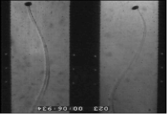
As path instability sets in, a bubble can either zigzag or spiral. For both cases, a double-threaded wake is observed. It is illustrative to analyze the zigzagging bubble as a separate case. As the motion is in one plane, a two dimensional flow analysis is possible. The results of this analysis also explain the apparent differences between the wake of a spiralling bubble and the wake of a zigzagging bubble.

In Figure 5 the two perpendicular views of a zigzagging bubble (req = 1.00 mm) can be seen. The motion of the bubble is in a single plane (two-dimensional); by coincidence, this plane coincides with one of the projection planes in this experiment. Figure 6 and 7 show the successive schlieren images of a bubble (req = 1.00 mm) in zigzagging motion. Each pair of images contains the XZ and YZ view, respectively. Note that in the YZ-view the path is straight while it is sinusoidal in the XZ-plane. The shape of the bubble appears to change significantly in the right view (compare t = 12 with t = 56 ms). This is not necessarily a shape oscillation as from the other view it is clear that the bubble can be moving towards or away from the observer, which for a flattened ellipsoid results in a change of the projection. In the left image the shape of the bubble is alsochanging (compare t = 52 with t = 68 ms) as in figures 6 and 7. This cannot be a result of the projection. It is concluded that there is a shape oscillation for zigzagging bubbles. In the experiments, this shape oscillation appeared to have the same frequency as that of the path. It is conjectured that the shape is related to the orientation and the nature, single- or double-thread, of the wake.

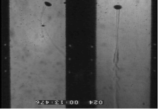Figure 5. The double-threaded wake behind a zigzagging bubble (req = 1.00 mm). By coincidence, the plane of the zigzag coincides with one of the views (A.W.G. de Vries 2001)

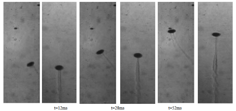Figure 6. Successive schlieren images of a bubble (req = 1.00 mm) in zigzagging motion. Each pair of images contains the XZ and YZ view, respectively. Note that in the YZ-view the path is straight while it is sinusoidal in the XZ-plane

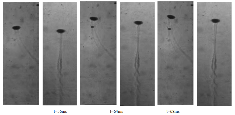Figure 7. Continuation of schlieren images of a zigzagging bubble. The wake of the bubble is a double-threaded wake, unless the curvature of the path iszero (starts at t ≈ 24 ms) in the mean position of the zigzag. The wake reconnects and in the following the occurrence of an instability is observed in the wake. It is clear that the zigzag is NOT maintained by vortex shedding at the maximum of the sinus in the XZ-plane (t ≈ 64 ms) (A.W.G. de Vries 2001)

Especially the wake shows very interesting phenomena. Just behind the bubble a double-threaded wake is visible in the YZ view of Figure 5. The left view of figure 5 only shows a single thread, caused by the projection; one thread blocks the view of the other thread. This is the general picture behind a zigzagging bubble: a double-threaded wake. However, when the bubble passes its ’mean’ position (t=28 ms) as in figure 6, or in other words, when the curvature of the path becomes zero, in both views only a single thread is observed. It is observed that the double-threaded wake only exists when the curvature of the path is nonzero. This is in agreement with the single-threaded wake observed for straight rising bubbles (A.W.G. de Vries 2001).

The patterns observed in the wake, several bubble diameters behind the bubble, are a result of the instability of the double-threaded wake. This is not vortex shedding, as was assumed by other researchers, e.g. (Lunde and Perkins 1997 and Br¨ucker 1999). For the bubbles in the present regime of interest, vortex shedding is not observed. (A.W.G. de Vries 2001) showed that the instability of the double threaded wake (two counter rotating vortex filaments) is in fact the Crow instability (Crow 1970). In general, this instability corresponds with the instability of the trailing vortices behind airplanes.

On the other hand, the turbulence structure of bubbly flows is one of the important subject matters in multi-phase flows. Since the bubbly flow has multitudinous scales of flow structures in complicated coexistence, it is necessary to approach systematically to the bubbly flow regarded as a hierarchy structure of multi-scales (Nakagawa et. al. 2007).

(Nakagawa et. al. 2001 and 2003) measured the velocity profiles around bubbles in bubbly flows using an Ultrasonic Velocity Profile monitor (UVP) within the limits of 400 < Re_B < 1200 in bubble Reynolds number and elucidated the existence of the boundary layer around each bubble and its characteristics. The bubble boundary layer has also the transition from laminar to turbulent. The critical bubble Reynolds numbers are Re_B,crit ≈ 1000 without the influence of leading bubbles and Re_B,crit = 600-750 under the influence of leading bubbles, respectively. In the bubble Reynolds number range considered, zigzag rising bubbles are observed in bubbly flows (Nakagawa et. al. 2007).

Zigzag rising motion of a bubble is a typical motion of bubbles in bubbly flows. Vortices shedding oscillatory behind a bubble and the wake of the bubble turning periodically similar to a sign of inequality are regarded as the most fundamental causes of the turbulence excited in bubbly flows, because these phenomena produce an alternating lift force (Nakagawa et. al. 2007).

(Nakagawa, et. al. 2006) had developed a spinning sphere model, which enable to treat more exactly with the actual lift production, and considered the lift production on a zigzag rising bubble trailing a hairpin vortex on photographic evidence. (Nakagawa et. al. 2007) explicated fluid-dynamically the alternating lift production on a rising originally nonspin bubble and the zigzag turning of its path, and proposed a chain process as a fluid-dynamic mechanism which produces rising bubbles zigzag motion.

(Nakagawa et. al. 2007) develop a novel concept and a universal model for the bubbly turbulent flow excited by zigzag rising bubbles as a complex system. They assume a buffet which is an elementary effect of the hairpin vortices shed periodically from the leading bubbles on the trailing ones in bubbly flows, and propose the chains of buffeting as the chain process where the leading bubble’s wake makes the trailing one’s boundary layer transit successively from laminar to turbulent. Therefore, they discuss the phase transition of complex system to the self-organizing critical structure by the above-mentioned buffet chains in bubbly flows as a model for bubbly turbulent flows (Nakagawa et. al. 2007).

3.1.3. Spiralling Bubble

The path of a spiralling bubble is hardly ever a perfect spiral. Observed from above the perfect spiral path would be a circle. Otherwise, ellipses are observed. For every spiralling bubble, a double-threaded wake was observed Figure 8. The three dimensions (3D) views were studied as 2 views, the first one located on the left side of the figure which is the XZ view where Z is the vertical direction and X is the horizontal direction. The second one is located on the right side of the figure that is the YZ view, where Z is the vertical direction while Y is the horizontal direction. When spiralling bubbles are small or close to perfectly spiralling this is a stable wake. For large bubbles and ellipsoidal top views of large aspect ratio (tendency towards zigzag), this wake is unstable close to the bubble. Although even for the perfectly spiralling bubble the wake becomes unstable a long time after the bubble has left the frame of view, this wake is called stable (A.W.G. de Vries 2001).

Figure 8. The two perpendicular views, XZ and YZ, of a double-threaded wake behind a nearly perfectly spiralling bubble (req = 1.01 mm)

For a stable bubble wake in both views it might appear that the filaments are twisting but this is a result of the projection. Care has to be taken in identifying spiralling or zigzagging from just one side view. Two views are needed, because often in one view a motion might look like a spiral, but appears to be a perfect zigzag.

From the separate views, a mode-2 axisymmetric shape oscillation appears to be present. However, after the bubble shape and orientation is recalculated with the analysis program, no shape oscillations of the bubble are found. For zigzagging bubbles, a mode-2 oscillation has been observed and has been related to the orientation and the nature of the wake. Contrary to zigzagging bubbles, the wake consists of a double-threaded wake at all times. For a spiralling bubble the orientation of the filaments is not changing relative to the orientation of the bubble. The bubble has a fixed shape, but the orientation changes in such a way that the minor axis is directed along the path (A.W.G. de Vries 2001).

The spiralling (also called helical) motions of axisymmetric solid bodies in a perfect fluid are well understood and described by (Lamb 1932). Solid bodies with angular inertia about their axis of symmetry have an infinite range of possible helical motions. Within a Hamiltonian description, a bubble in spiralling motion has to have a non-zero impulsive couple. With the use of a variation characterization, the path of bubbles can be determined within the Hamiltonian theory developed by (Benjamin 1987). In this theory, it is assumed that the ideal-fluid theory is applicable for the motion of bubbles including surface tension in liquids of small viscosity. In the region in which the Weber number is decisive for stability, the ideal-fluid model has been proven to be a valid assumption by e.g. (Saffman 1956, Hartunian and Sears 1957, Moore 1965 and Miksis et al. 1981).

The configuration of the wake behind drops was extensively studied by (Magarvey and Bischop 1961) and for small drops they also observed a single-threaded wake. The transition towards a double-threaded wake occurs already at Re =210, which is comparable to the critical Reynolds number for solid spheres. However, for both drops and solid falling spheres no path instability has been observed. This is probably caused by the difference in the moments of inertia (Ryskin and Leal 1984). The rotation of the wake of a solid light sphere (Achenbach 1974) eventually induces the sphere to follow a spiralling path and to reduce the terminal rise velocity (Karamanev et al. 1996).

3.2. The Wake

Close to the bubble the spiralling and zigzagging wake (Figures 9 and 10) are in general similar, although they show great differences in their subsequent behavior. The wake of zigzagging bubbles is unstable on a short time-scale, whereas the instability of the wake of a spiralling bubble sets approximately 2s later. The instability in the wake can be explained by the tendency of the counter-rotating vortex filaments to become unstable. In case the structure of the bubble wake is comparable with the wake of an airplane, the wake of the bubble is susceptible to the Crow instability. In (Crow 1970) pictures of the pair of counter rotating trailing vortices of an airplane in cruise Figure 9 are shown. In these pictures, the instabilities are clearly observable (A.W.G. de Vries 2001).

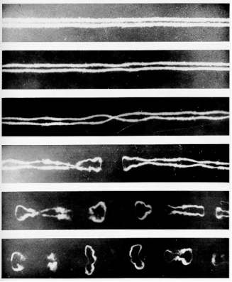Figure 9. The Crow instability of the trailing vortices in the wake of a B-47 at cruising speed and altitude. (Taken from Smith and Beesmer 1959)

Figure 10. Multiscale structure of bubbly flows in aqueous surfactant solution

Extensive research (e.g. Widnall et al. 1971) showed that an initial small perturbation is the onset of this instability. For a zigzagging bubble the initial perturbation, the reconnection of the vortex filaments, is larger than for a spiralling bubble with a regular wake. Therefore, the instability develops much quicker and is already visible close to the bubble. For the spiralling bubble this instability occurs about 2s after the vortex pair was generated on the bubble. This is equivalent to about 300 bubble diameters behind the bubble. Similarly, for airplanes this instability would set in several hundreds of wing-spans behind the airplane (A.W.G. de Vries 2001).

A path and wake visualization method has been developed by (A.W.G. de Vries 2001) that does not affect the purity of the water. It was found that the wake of spiralling and zigzagging bubbles consists of two counter-rotating vortex filaments. Both motions are in many aspects similar and can occur for roughly the same experimental conditions.

The differences seen in the configuration of the wake far behind the bubbles can be explained by instability of the system of the two counter-rotating vortex filaments. As the initial disturbance of the wake for a zigzagging bubble is larger than for a perfectly spiralling bubble, this instability is observed closer to the bubble. The wavelength of this instability is much smaller than the wavelength of the bubble’s motion. Consequently, this instability cannot be the explanation for the zigzag motion of a bubble in pure water.

As soon as the curvature of the path becomes non zero the wake consists of a double-thread vortex system. This double-thread is shown to be associated with a lift force on the bubble. The perfect two-dimensional motion for a zigzag can be explained by taking the lift force into account. The lift force is always directed perpendicular to the path.

The wake of zigzagging bubbles consists of a double-threaded wake as long as the curvature is non-zero. When the curvature becomes zero the vortex filaments reconnect and successively a double-threaded wake of consisting of two counter rotating vortex filaments of opposite sign is formed.

A lift force can be associated with the double-threaded wake. The strength of this lift force can be obtained from the self-induced motion of the wake, the force needed to maintain the spiralling motion, or from a balance between buoyancy and lift force as soon as the curvature of the path becomes zero for a zigzagging bubble.

Since all experiments reported by other authors concluded that vortex shedding (similar to the case of solid spheres) is the mechanism for the zigzag motion, the purity of the water used in their experiments is questionable. Yet, in many cases, the water was still considered clean, based on measurements of the rise velocity of the bubble. Consequently, a better indicator for the purity of the water should be used. A temperature gradient has an effect on the rise velocity of the bubble; nonetheless, it does not affect the purity of the water.

Furthermore, shape oscillations have not been observed for spiralling bubbles. The mode-2 shape oscillation claimed by other researchers, is in fact, a result of the limited information on the bubble’s shape when considering only a single projection. A more detailed analysis employing two projections shows no shape oscillations. For zigzagging bubbles, a shape oscillation is observed and is related with the disappearance and reappearance of the double-threaded wake (A.W.G. de Vries 2001).

On the other hand, experimentally the study of bubble wakes has been mainly performed by dye visualization (Lunde and Perkins 1997), LDA (Ellingsen and Risso 1998) or by PIV (Br¨ucker 1999). In these studies, vortex shedding is observed for zigzagging bubbles, similar as is observed for solid spheres. For spiralling bubbles, (Lunde and Perkins 1997) observed a double threaded wake and emphasized that this would consist of two counter rotating vortex filaments. To resolve the wake with these techniques a large amount of particles/dye is needed. It is most likely that these techniques contaminate the water; the validity of these results for clean water is questionable. Contamination might explain the similarity of the wake structure for these zigzagging bubbles and that of numerically; especially the works of (Ryskin and Leal 1984 a, b, Takagi et al. 1997 and Blanco and Magnaudet 1995) are interesting, because they all report on the formation of an attached, or standing, eddy behind a strongly deformed bubble. Ryskin and Leal concluded that for vortex shedding to occur with clean bubbles two conditions have to be satisfied: i) a standing eddy behind the bubbles, and ii) We > We_cr. From the numerical work of (Blanco and Magnaudet 1995 and McLaughlin 1996), however, it can be deduced that no standing eddy will exist behind a bubble in the regime in which, experimentally, path instability occurs in pure water. This leads to a contradiction since without a standing eddy, vortex shedding will not occur. Some experiments reported that indeed another mechanism is observed for zigzagging bubbles.

For a better understanding of the dynamics of wakes, and especially the behavior of bubble wakes, the studies of wakes behind solid spheres and drops by (Achenbach 1974, Magarvey and Bischop 1961, Natarjan and Acrivos 1993 and Johnson and Patel 1999) are very informative.

The drag coefficient of solid spheres and drops is generally larger than for bubbles; this behaviour is related to the amount of vorticity produced. For larger bubbles, though, the deformation might become so large that the drag coefficient will be larger than the drag coefficient of a solid sphere of the same volume. Furthermore, it is observed that the drag coefficient of light solid spheres differs from that of heavy solid spheres (Karamanev et al. 1996). In (A.W.G. de Vries 2001) work light particles are observed to spiral in a manner similar to some bubbles.

The experimental results of (Magarvey and Bishop 1961) for the wake behind drops come closest to what is observed for wakes behind bubbles. At low Reynolds numbers, the wakes of drops and bubbles are very similar, consisting of a single thread. For slightly larger Reynolds numbers, both feature a double threaded wake. At very large Reynolds numbers, an intermittent wake is observed for both the drop and the bubble. However, for the intermediate regime, in which path instability sets in for bubbles in pure liquids, the observations of the wake behind bubbles, drops, and solids are very different.

(Natarjan and Acrivos 1993) reported on the stability of the axisymmetric flow around solid spheres and disks obtained in numerical simulations. They concluded that two different instabilities could occur at two distinct critical Reynolds numbers. The first critical Reynolds number, observed for spheres and disks, was associated with the instability of the near wake. The second critical value of the Reynolds number indicated a periodic instability or waviness of the far wake. They emphasized that for different objects the second instability might be reached at a lower Reynolds number than the first instability, and so the mechanism for the observed instability, might change (A.W.G. de Vries 2001).

3.3. Contamination and Marangoni Effects

The behavior of bubbles changes significantly as soon as fluids become contaminated with surfactants. This change is related to the fluid properties and the type and level of contamination. (Haberman and Morton 1954) showed that for contaminated water the critical radius, where the first path instability sets in, decreases, as does the maximum rise velocity and Re_cr. (Hartunian and Sears 1957 and Ryskin and Leal 1984 a, b) showed that, for a contaminated system, the stability curve is not determined by a critical Weber number but by Re_cr = 200, as is observed for solid spheres. (Bel Fdhila and Duineveld 1996) determined that the rise velocity of a bubble stays roughly equal to its value for pure fluid up to a critical surfactant concentration. Above this concentration, the drag rapidly increases towards the solid sphere drag. They also observed the transition for the path instability at Re = 203 for contaminated bubbles.

(McLaughlin 1996) adapted the numerical method of (Ryskin and Leal 1984) to take into account contamination. For the pure water case comparison with (Duineveld 1995) was made and no attached wake was observed for Re=637 and We=3.17. In none of the simulations for clean interfaces flow separation was observed. For contaminated water a standing eddy is already observed for Re=110, We=0.166 and flow separation is observed. This clearly shows the differences in the wake behind bubbles in pure and contaminated water (A.W.G. de Vries 2001).

Small amount of surfactant can drastically change bubble behaviors. For example, it is well known that a bubble in aqueous surfactant solution rises much slower than one in purified water. This phenomenon is explained by the so-called Marangoni effect caused by a surface concentration distribution of surfactant along the bubble surface. In other words, a variation of surface tension appears along the surface due to the surface gradient of surfactant concentration, and this causes a tangential shear stress on the bubble surface. This shear stress results in the decrease of the rising velocity of the bubble. This Marangoni effect influences not only the rising velocity, but also any other behaviors such as zigzag/spiral motion of bubbles in quiescent water (Magnaudet and Eames, 2000) and its transition and lateral migration in the presence of mean shear. The recent studies related to these interesting behaviors of bubbles caused by the surfactant adsorption/desorption on the bubble surface were reviewed by (Yoshiyuki et. al. 2010). Surfactant effects on single bubble motion in quiescent water and upward bubbly flow in a rectangular channel are investigated by (Yoshiyuki et. al. 2010). Generally, path instability of the single bubble and the bubble motion in inhomogeneous flow are sensitive to the contamination of water. Addition of surfactant in gas-water system yields immobilization of the bubble surface due to Marangoni effect. Single bubble 3D trajectories in dilute surfactant solution are measured by two high-speed cameras. All measured trajectories are plotted on two dimensional field of bubble Reynolds number Re and instantaneous boundary slip condition. In free-slip and no-slip condition, bubble motions are dependent on Re. However, in half-slip condition, bubble motions are spiral and almost independent from Re. Bubbles in certain condition move along trajectories changing from spiral to zigzag. These interesting motions are caused by changing slip condition. Bubble motion in upward channel flow is also observed. The local void fraction distribution changes from wall-peaking to uniform by stronger Marangoni effect. This is because that shear-induced lift force on 1 mm spherical bubble decreases due to the change of the boundary condition of the bubble surface from free-slip to no-slip, and the tendency of the lateral migration toward the wall becomes weaker (Yoshiyuki et. al. 2010).

Furthermore, these phenomena influence the multiscale nature of bubbly flows and cause a drastic change in the bubbly flow structure as shown in Figure 10. In this talk, related to these interesting multiscale structures, bubble clustering phenomena in upward bubbly channel flows are discussed with the emphasis on the detail description of a single bubble behavior influenced by the surfactant adsorption/desorption kinetics on the bubble surface (Takagi and Matsumoto 2011).

Even if a bubble remains quite spherical, it can experience forces due to gradients in the surface tension, S, over the surface that modify the surface boundary conditions and therefore the translational velocity. These are also called Marangoni effects. The gradients in the surface tension can be caused by a number of different factors. For example, gradients in the temperature, solvent concentration, or electric potential can create gradients in the surface tension.

The thermo capillary effects due to temperature gradients have been explored by a number of investigators (for example, Young et, al., 1959) because of their importance in several technological contexts. For most of the range of temperatures, the surface tension decreases linearly with temperature, reaching zero at the critical point. Consequently, the controlling thermo physical property, dS/dT, is readily identified and more or less constant for any given fluid.

Surface tension gradients affect free surface flows because a gradient, dS/ds, in a direction, s, tangential to a surface clearly requires that a shear stress act in the negative s direction in order that the surface be in equilibrium. Such a shear stress would then modify the boundary conditions for example, the Hadamard-Rybczynski conditions, thus altering the flow and the forces acting on the bubble.

As an example of the Marangoni effect, the steady motion of a spherical bubble in a viscous fluid was examined when there exists a gradient of the temperature (or other controlling physical property). Much more realistic is the assumption that thermal conduction dominates the heat transfer and that there is no heat transfer through the surface of the bubble.

For simplicity, the bubble is assumed to remain spherical. This assumption implies that the surface tension differences are small compared with the absolute level of S and that the stresses normal to the surface are entirely dominated by the surface tension.

In addition to the normal Hadamard-Rybczynski drag (first term), a Marangoni force can be identified, acting on the bubble in the direction of decreasing surface tension.

Finally, a related effect caused by surface contaminants that increase the surface tension should be clarified. When a bubble is moving through liquid under the action, say, of gravity, convection may cause contaminants to accumulate on the downstream side of the bubble. This will create a positive dS/dθ gradient that, in turn, will generate effective shear stress acting in a direction opposite to the flow. Consequently, the contaminants tend to immobilize the surface. This will cause the flow and the drag to change from the Hadamard-Rybczynski solution to the Stokes solution for zero tangential velocity. The effect is more pronounced for smaller bubbles since, for a given surface tension difference, the Marangoni force becomes larger relative to the buoyancy force as the bubble size decreases. Experimentally, this means that surface contamination usually results in Stokes drag for spherical bubbles smaller than a certain size and in Hadamard-Rybczynski drag for spherical bubbles larger than that size. Such a transition is observed in experiments measuring the rise velocity of bubbles and can be seen in the data of (Haberman and Morton 1953, Harper and Pearson 1967, Moore 1963, 1965) have analyzed the more complex hydrodynamic case of higher Reynolds numbers (Christopher 2005).

As a result, it is clear that any small change in surface type and shape can significantly affect the behavior of bubbles in fluid flow. Marangoni effect explains a well known phenomenon about bubbles motion on surfaces. This phenomenon state that a bubble in aqueous surfactant solution rises much slower than one in purified water. Two kinds of experiments are conducted; Marangoni effect which is caused by a surface quiescent surfactant solution and the other is a concentration distribution of surfactant along upward turbulent bubbly flow in a vertical the bubble surface (Magnaudet and Eames, 2000).

3.4. Bubble-bubble and Bubble-wall Interactions

The interaction between two bubbles has been studied by (Biesheuvel and Van Wijngaarden 1984, Kok 1993a, b and Duineveld 1994). (Van Wijngaarden 1993) performed potential flow calculations on a collection of small spherical air bubbles. (Duineveld 1994) determined a critical Weber number for the transition between coalescence and bouncing, which is We_cr = 0.18 based on the approach velocity. At a We_cr of 2.6, based on the rise velocity, there is a transition between bouncing and bouncing followed by separation. Duineveld observed coalescence, bouncing, and bouncing separation for different bubble sizes. The minimum bubble size for bouncing separation (0.86 mm) is close to the critical size for path instability (0.91 mm). He argued that this size could be slightly lower because the large distortion at the bounce triggers vortex shedding, which he assumed to be the cause of zigzag motion. (A.W.G. de Vries 2001).

3.4.1. Shape Effects

The way a bubble is produced can be very important for its subsequent behavior. Especially bubble shape oscillations at the moment of release of bubbles should be avoided. Furthermore, small deviations of the exact shape can have a tremendous effect on the flow around the bubble.

For the study of path stability, it is desirable to eliminate as many sources of disturbances as possible. Possible source of disturbances are volume and shape oscillations triggered at the production and release of the bubble. These can be eliminated. The bubble production apparatus used in the (A.W.G. de Vries 2001) experiments is developed for accurate, reproducible bubble sizes in a large range of sizes, and it has the advantage that initial bubble shape oscillations are not observed. In the experiments, the needles (capillaries) are small and well polished, which has a positive effect on the smoothness of the release.

The shape and the orientation of the bubble can have significant effects on the flow around the bubble. Numerically it will be shown that a small deviation of the bubble’s ellipsoidal shape delays the formation of a standing eddy. Furthermore, theses numerical simulations indicate that at the onset of path instability in experiments, a standing eddy does not exist behind a bubble (A.W.G. de Vries 2001).

3.4.2. Bubble Release

For the study of path instability of a free rising bubble, external factors influencing the stability should be eliminated. One very important factor is the bubble formation and its release. This should be as smooth as possible. Ideally the aim is to release a single exactly spherical bubble, without any shape oscillations, in totally quiescent pure water (A.W.G. de Vries 2001).

3.4.3. Shape Effects on the Flow Pattern

The consequences of the shape deformation on the flow around the bubble can be considerable. In (A.W.G. de Vries 2001) study numerical simulations, using the code of (Takagi et al. 1994), have been performed. The simulations are grid independent. Two results are presented by (A.W.G. de Vries 2001). Both calculations, with equally sized bubbles, are performed taking into account a zero tangential stress condition at the bubble surface. In the upper half the bubble shape is fully adjustable and in the lower half the bubble shape remains an ellipsoid. Nevertheless the effects on the flow around the bubble are large. For the fully adjustable, axisymmetric shape, no recirculation zone is observed, whereas for the fixed ellipsoidal shape such a zone is clearly visible. It is concluded that calculations assuming a fixed, ellipsoidal shape do not lead to physically correct velocity fields.

3.4.4. Bubble-Wall

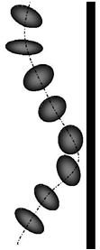
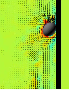
The flow characteristics of a dispersed multiphase flow, such as a bubbly flow and a solid-liquid two-phase flow, are influenced by the interactions between the particle or bubble and its surrounding fluid, and among the particles, and between the particle and a wall. Therefore, investigation of these interactions is important to understand the flow characteristic of a dispersed multiphase flow. A particle-fluid and particle-particle interactions by using MOFIA (Moving-Object and Fluid Image Analyzer) which consist of PIV for velocity measurement and stereo image processing for particle behavior was studied. The interaction between a bubble and the wall was investigated experimentally (Hideaki and Kar-Hooi 2007). The experiment was done for a single bubble rising near the wall of a riser and the bouncing motion of the bubble was measured by the stereo image processing in the MOFIA. The bubble of about 2 mm diameter moved toward the wall by the lift force due to the velocity gradient of the water flow. After touching the wall, the bubble bounced and moved toward the center of the pipe but again turned to the wall due to the lift force (Hideaki and Kar-Hooi 2007).

In the measurement, the three-dimensional bubble shape was reconstructed based on the stereo image under the assumption of the oblate steroidal shape. The assumption was proper for a bubble affected by a drug force along the moving direction from the surrounding liquid. In the image processing, the three-dimensional position and aspect ratio (minor axis length / major axis length) of the bubble can be obtained. Furthermore, the orientation of the bubble or the direction of the minor axis can be also known (Hideaki and Kar-Hooi 2007).

The experimental results showed the deformation, orientation and velocity of the bubble during the bouncing process. Figure 11 shows the typical bouncing motion of a bubble based on the measurement. The bubble shape was an oblate spheroid and the minor axis of the bubble was parallel to its moving direction before touching the wall, which was supposed as the effect of the drag force of the water. After touching the wall, the minor axis was not parallel to the moving direction. The aspect ratio changed during the bouncing motion. Just after touching the wall, the bubble shape approached to the spherical and became oblate spheroid again as leaving from the wall (Hideaki and Kar-Hooi 2007).

Figure 11. Typical bouncing motion of a bubble

The bouncing motion was repeated periodically in the narrow space near the wall. The phenomenon was related to the energy supply from the lift force due to the water velocity. The restitution coefficient was estimated as one or more. The reason was not clear but the surrounding liquid motion was an important role as shown in Figure 12 obtained by MOFIA and showing the velocity field around the bubble. Figure 12 shows the upward motion of the water at the top of the bubble and also the motion flowing into the gap between the bubble and the wall at the bottom of the bubble.

Figure 12. Velocity fields around a bubble bouncing on the wall

As mentioned above, the characteristics of bubble behavior bouncing on the wall were shown clearly based on the experimental results (Hideaki and Kar-Hooi 2007).

Furthermore, issues connected with the presence of a vertical wall and bubble movement around it are important in two-phase flows analysis. An experimental data on the flow resistance of gas bubbles near vertical walls as well as mathematical description of that problem was produced by (Dariusz and Jan 2007). Hence; the aim of their work was investigation focused on accurate experimental verification of forces acting on a model of a bubble flowing along the wall. In their study, the bubble is represented by a solid sphere suspended on a thin string. It is acknowledged that bubbles in motion near the wall exhibit some more specific patterns of motion, however, the model of a bubble motion captures at least a qualitative behavior of a bubble in the flow and will compliment understanding of transverse force balance on the bubble. In general, the wall causes the bubbles to slow down, in both the parallel and the transverse direction with respect to wall alignment. Obtained experimental results have been confronted with correlations due to (Antal 1991 and Tomiyama 1998). A good consistency between correlations taken from literature and mathematical model confirms the appropriateness of assumptions used in (Dariusz and Jan 2007) study. Data collected in the course of experiments has been reduced to yield a general form of a correlation, which enables determination of the “wall effect” (Dariusz and Jan 2007).

Bubbles bouncing against vertical walls have been studied experimentally. Many experiments including (A.W.G. de Vries 2001) are performed in water of 20^◦C, and thus only the path of the bubbles is recorded. Furthermore, experiments with a temperature gradient are reported to indicate the observations in the wake and during bouncing. Based on the experimental results a model is proposed by (A.W.G. de Vries 2001) to explain the variety of observed bubble paths. Crucial for this model are the bouncing criteria and for larger bubbles wake effects.

The motion of two interacting bubbles has been studied extensively by (Kok 1989, 1993a, b and Duineveld 1994). Two bubbles tend to align horizontally and attract each other. At close approach there are various possibilities:

i) coalescence,

ii) repeated bouncing followed by coalescence

iii) bouncing followed by separation.

The observed motions depend on the fluid properties, the initial distance and the size of the bubbles. (Duineveld 1994) determined experimentally the critical Weber number for the transition from one type to the other. The motion of the bubble pair after bouncing was explained satisfactorily by (A.W.G. de Vries 2001).

In inviscid flow theory, the effect of a wall on a bubble can be modeled by mirror-imaging the bubble in the wall, i.e. leading to a bubble pair. Coalescence does not occur for a bubble bouncing against a vertical wall. Also the boundary layer, built up during bouncing, is different from the situation for a bubble pair. However, experimentally a bubble-wall interaction is more convenient because the ’bubbles’ are necessarily identical and aligned horizontally. In potential flow theory, the attraction is captured, but the remarkable bouncing phenomena observed in experiments are not predicted.

Depending on the size of the bubble and the initial distance to the wall, the bubble may slide along the wall, perform multiple rebounds or rebound once without returning to the wall. Often the rebound amplitude is larger than the initial distance to the wall. Although energy is dissipated by drag, the amplitude of the rebounds will not damp for multiple bounds.

One of the few studies on bubbles interacting with walls was performed by (Tsao and Koch 1997). They focussed on surface energy and the effect of deformation of a bubble rising underneath an inclined or horizontal plate. They claim that at the collision immediately up to 95% of the energy contained in the initial kinetic and surface energy is converted in surface deformation. After the rebound a significant fraction (up to 59%) of the bubble’s energy is lost and most of this loss occurred just after the collision. They proposed two mechanisms: acoustic radiation and, just after the collision, separation of the boundary layer at the wall.

(A.W.G. de Vries 2001) suggested that the vorticity built up in the wake of the bubble plays an important role. To study this, a similar setup and visualization technique is used and a model is proposed to explain the motion of the bouncing bubble. The global path of the bubble is experimentally studied with a diffusive side lighting technique (A.W.G. de Vries 2001).

3.4.5. Collision

In the experiments, the vertical velocity drop for bouncing bubbles is observed to occur in a few milliseconds. In the model, this drop is assumed to occur instantaneously.

As soon as the bubble hits the wall (x ≤ req) the Weber number based on the approach velocity is calculated, which determines the type of bounce: for We < We_cr sliding along wall (u→−u, v → v), for We ≥ We_cr, bouncing (u→−u, v → 0). In the first case the potential flow solution, including drag, of a bouncing bubble is applicable; soon the bounce amplitude is damped by dissipation. In the bouncing case, the vertical velocity component becomes very small (in the model zero) which immediately decreases the bubble attraction force, which is proportional to the velocity squared. In general v >> u just before bouncing (A.W.G. de Vries 2001).

The bouncing case may be interpreted as a mass-spring system consisting of many equivalent springs. Initially the springs are stretched and the velocity of the mass is zero. Subsequently the mass accelerates till the springs reach their rest length. At that moment, the mass is moving with a velocity of u and bounces elastically with a wall. The velocity becomes −u. At that time, the springs are cut all. This results in a lower spring constant and enables a larger stretch of the spring than the initial one. After a while all the springs are reconnected to the mass and thus the spring constant is increasing. The rest length has not changed. The bubble returns towards the rest length and at that moment, the same bounce occurs again. Without drag the velocity at this time is larger than u and the consecutive stretching is increased again and again. With drag the maximum stretch length is bounded as is the bounce amplitude of a bubble bouncing with a vertical wall. For the bouncing bubble, the attraction force is changing in a similar way as the force for the different springs. Admittedly the springs are very peculiar as the force each spring exerts on the mass is decreasing as the spring is further stretched (A.W.G. de Vries 2001).

3.4.6. After collision

After the bounce, the motion of the bubble can again be described by the equations of motion. In case of sliding, the bounce height will become zero almost instantaneously. For a bouncing bubble, the vertical velocity is reduced significantly and thus the attraction force becomes negligible. The bubble bounces away from the wall and gravity will accelerate the bubble again towards its terminal velocity. The attraction force is increased and the bubble will experience another bounce. The maximum distance to the wall can be larger than the initial distance to the wall (A.W.G. de Vries 2001).

Bouncing phenomena can be approximately described by a model based upon potential flow, taking into account bouncing criteria and wake effects. The larger bounce amplitude than the initial distance to the wall can be explained with this model. The attraction force of a bouncing bubble reduces significantly, as the bubble vertical velocity component drops. At bouncing, the horizontal momentum is conserved. The combination of both makes a larger bounce possible or can compensate for the energy loss by dissipation (A.W.G. de Vries 2001).

One of the questions still remaining is the slowing down of the bubble after bouncing. It is assumed that the wake of the bubble and its vorticity first pushes itself in between the wall and the bubble. The further development of the wake shows a down-flow region near the bubble, which is probably causing the bubble to slow down. Furthermore, the vortical blob formed will have an attraction force, being able to hold the bubble near the wall. This force quickly drops to zero as the distance between the bubble and vortical blob increases.

It is observed that as soon as ellipsoidal bubbles hit the wall they immediately become spherical. More research is needed to estimate the effects of deformation on the bouncing phenomena, especially for the large bubbles. Although the lift force related to the wake can explain the rebounds and the amplitude of the bounce, the path of the bouncing bubble cannot be reproduced accurately for the large bubbles (A.W.G. de Vries 2001).

3.4.7. Pseudo-Turbulence in Bubbly Flows

Bubbles rising in turbulent flows will affect this flow and introduce velocity fluctuations. This phenomenon is called “pseudo-turbulence”. Following the first tentative explanation of (Van Wijngaarden 1998) based on potential flow theory around nonspherical bubbles with thin boundary layers, (A.W.G. de Vries 2001) model Hill’s Spherical Vortices as an extra source of turbulence. These vortices are assumed to be shed from the rising bubbles ’hitting’ turbulent regions in a similar way as observed in their experiments on a bubble bouncing against a vertical wall. A significant contribution of these vortices is observed. Furthermore, this model is extended to take into account the effects of the rearrangement of vorticity in the wake of the bubble (A.W.G. de Vries 2001).

In bubbly flows, there is a two-way coupling between bubbles and turbulence. Turbulence affects the trajectories of the bubbles and bubble motion introduces velocity fluctuations, and therefore Reynolds stresses, in the liquid. This process is called pseudo-turbulence. The term turbulence refers to the fluctuating character of the flow, the term “pseudo” indicates that the origin of the turbulence is an induced motion by the bubbles.

The importance of pseudo-turbulence is emphasized by experiments of (Lance and Bataille 1991, Henderson and Miles 1994 and Theofanous and Sullivan 1982).

(A.W.G. de Vries 2001) analysis showed the considerable effect of vorticity generated by the bubbles on the excess turbulent energy. The experimental results of (Lance and Bataille 1991 and Theofanous and Sullivan 1982) are within the upper and lower bound of the model. The lower bound of this model is given by the natural frequency of a single rising bubble in quiescent water. The upper bound is given by the maximum amount of vorticity produced on the surface of the bubble in quiescent water.

In the model, the vorticity is concentrated in Hill’s spherical vortices. Admittedly, this is not necessarily so in the real situation. It is expected, however, that the excess energy will be of the same order of magnitude as estimated in the analysis of (A.W.G. de Vries 2001).

3.4.8. Deformation Due to Translation

Since the fluid stresses due to translation may deform the bubbles, drops or deformable solid particles that make up the disperse phase, we should consider not only the parameters governing the deformation but also the consequences in terms of the translation velocity and the shape. The author concentrates on bubbles and drops in which surface tension, S, acts as the force restraining deformation (Christopher 2005).

3.4.9. Bjerknes Forces

Another force that can be important for bubbles is that experienced by a bubble placed in an acoustic field. Termed the Bjerknes force, this non-linear effect results from the finite wavelength of the sound waves in the liquid. The form of the primary Bjerknes force produces some interesting bubble migration patterns in a stationary sound field (Christopher 2005).

3.4.10. Growing or Collapsing Bubbles

When the volume of a bubble changes significantly, that growth or collapse can also have a substantial effect upon its translation. A bubble that grows or collapses close to a boundary may undergo translation due to the asymmetry induced by that boundary. A relatively simple example of the analysis of this class of flows is the case of the growth or collapse of a spherical bubble near a plane boundary, a problem first solved by (Herring 1941, Davies and Taylor 1942, 1943). Assuming that the only translational motion of the bubble is perpendicular to the plane boundary with velocity (Christopher 2005).

Unlike solid particles or liquid droplets, gas/vapor bubbles can grow or collapse in a flow and in doing so manifest a host of phenomena with technological importance.

3.5. Cavitation

Cavitation occurs in flowing liquid systems when the pressure falls sufficiently low in some region of the flow so that vapor bubbles are formed. (Reynolds 1873) was among the first to attempt to explain the unusual behavior of ship propellers at higher rotational speeds by focusing on the possibility of the entrainment of air into the wakes of the propellor blades, a phenomenon we now term ventilation. He does not, however, seem to have envisaged the possibility of vapor-filled wakes, and it was left to (Parsons 1906) to recognize the role played by vaporization. He also conducted the first experiments on cavitation and the phenomenon has been a subject of intensive research ever since because of the adverse effects it has on performance, because of the noise it creates and, most surprisingly, the damage it can do to nearby solid surfaces (Christopher 2005).

Bubble flow interaction can be important in many practical engineering applications. For instance, cavitation is a problem of interaction between nuclei and local pressure field variations including turbulent oscillations and large scale pressure variations. Various types of behaviors fundamentally depend on the relative sizes of the nuclei and the length scales of the pressure variations as well as the relative importance of bubble natural periods of oscillation and the characteristic time of the field pressure variations. Similarly, bubbles can significantly affect the performance of lifting devices or propulsors. Some fundamental numerical studies of bubble dynamics and deformation, a practical method using a multi-bubble Surface Averaged Pressure (DF-Multi-SAP) to simulate cavitation inception and scaling were present by (Georges 2008), and connect this with more precise 3D simulations. This same method is then extended to the study of two-way coupling between a viscous compressible flow and a bubble population in the flow field (Georges 2008).

Study of cavitation inception teaches us that liquids rarely exist under a pure monophasic form and that bubble nuclei are omnipresent. These nuclei are very difficult to eliminate and are always in any industrial liquid at least in very dilute concentrations. However, most engineering studies, and rightfully so, ignore the presence of this very dilute often invisible bubble phase, and consider only the liquid phase to conduct analytical or numerical simulations. This applies to benign situations where pressure variations are not significant and where cavitation, dynamic effects, gas diffusion, and heat transfer do not result in dramatic modification of the flow to warrant inclusion in the modeling of both phases. In this contribution, those conditions should be considered and concerned where it is important to either evaluate whether cavitation may occur and/or to model the flow in presence of bubbles in significant local concentrations, sizes, or numbers to play a significant role in the flow dynamics. Under these conditions, interaction between the bubbles and the flow can be significant and need to be properly addressed. Three families of situations can be distinguished:

1. Cavitation Inception in uniform or acoustic flow fields

2. Cavitation Inception in vortical flow fields

3. Developed cavitation and bubbly flows.

In the first two cases, especially if cavitation inception is determined acoustically (i.e. prior to bubbles becoming visible,) the interaction between bubbles and liquid flow is ‘one-way’, i.e. the liquid dynamics affects the bubble dynamics, while bubble effects on the hydrodynamic flow field are negligible. In the third case, bubbles presence and behaviour is influential enough to affect significantly the basic flow field and implementation and use of ‘two-way’ interaction models is warranted.

The study of bubble dynamics in non-uniform flow fields is fundamental to the ability to predict or explain any cavitation effects in real flow fields. Recent contributions towards the fundamental understanding of bubble dynamics in non-uniform flow fields when large bubble deformations and bubble interactions are taken into account and described by (Georges 1994). A 3D Boundary Elernent Method is developed to describe the non-spherical bubble dynamics of each bubble in the flow, incorporating the influence of the underlying flow field which can be viscous. The method is used to study bubble dynamics in relatively simple fundamental flow fields such as the dynamics of bubbles in a shear flow near a flat wall, or in the flow field of a vortex line. It is then shown that bubble splitting, shearing of and development of surface instabilities are probably as common as the classical reentering jet formation (Georges 1994).

On the other hand, the direct numerical simulation (DNS) method has been used to the study of the linear and shock wave propagation in bubbly fluids and the estimation of the efficiency of the cavitation mitigation in the container of the Spallation Neutron Source liquid mercury target. The DNS method for bubbly flows is based on the front tracking technique developed for free surface flows. Thee front tracking hydrodynamic simulation code FronTier is capable of tracking and resolving topological changes of a large number of interfaces in two- and three-dimensional spaces. Both the bubbles and the fluid are compressible. In the application to the cavitation mitigation by bubble injection in the SNS, the collapse pressure of cavitation bubbles was calculated by solving the Keller equation with the liquid pressure obtained from the DNS of the bubbly flows. Simulations of the propagation of linear and shock waves in bubbly fluids have been performed, and a good agreement with theoretical predictions and experiments has been achieved. The validated DNS method for bubbly flows has been applied to the cavitation mitigation estimation in the SNS. The pressure wave propagation in the pure and the bubbly mercury has been simulated, and the collapse pressure of cavitation bubbles has been calculated. The efficiency of the cavitation mitigation by bubble injection has been estimated. The DNS method for bubbly flows has been validated through comparison of simulations with theory and experiments. The use of layers of nondissolvable gas bubbles as a pressure mitigation technique to reduce the cavitation erosion has been confirmed (Tianshi et. al. 2007).

3.5.1. Key Features of Bubble Cavitation

A) Cavitation inception

B) Cavitation bubble collapse

C) Shape distortion during bubble collapse

D) Cavitation damage

3.5.1.1. Cavitation Inception

Cavitation and bubble dynamics have been the subject of extensive research since the early works of (Besant in 1859 and Lord Rayleigh in 1917). A host of papers and articles and several books (Knapp et. al. 1970, Hammitt 1980, Young 1989, Franc et. al. 1995, Brennen 1995, Isay 1981, Leighton 1994 and Plesset 1964) have been devoted to the subject. Various aspects of the bubble dynamics have been considered and included one or several of the physical phenomena at play such as inertia, interface dynamics, gas diffusion, heat transfer, bubble deformation, bubble-bubble interaction, electrical charge effects, magnetic field effects, …etc. Unfortunately, very little of the resulting knowledge has succeeded in crossing from the fundamental ‘research world’ to the ‘applications world’, and it is uncommon to see bubble dynamics analysis made or bubble dynamics computations conducted for example by propeller or pump designers. This is due to the perceived impracticality of using the methods developed but for ‘experts’. However, with the tremendous advances in computing resources, these communities now commonly use Navier Stokes solvers and CFD codes to seek better solutions (Hsiao and Pauley 1999, Chahine 2004, Choi and Chahine 2006, Chen and Stern 1998 and Gorski 2002). The challenge is thus presently for the cavitation/bubble community to bring its techniques to par with the single phase CFD progress. Consideration of bubble dynamics within a CFD computation should also become common practice. Indeed, the tools already developed are at the reach of all users and should be adopted as more CFD tools to use for advanced design (Chahine 2004 and Choi and Chahine 2006).

3.5.1.2. Cavitation Bubbles

3.5.1.2.1. Observations of Cavitating Bubbles

Pioneering observations of individual cavitation events were made by Knapp and his associates at the California Institute of Technology in the 1940s (see, for example, Knapp and Hollander 1948) using high-speed movie cameras capable of 20,000 frames per second. Shortly (Thereafter Plesset 1949, Parkin 1952), and others began to model these observations of the growth and collapse of traveling cavitation bubbles using modifications of Rayleigh’s original equation of motion for a spherical bubble (Christopher 2005).

3.5.1.2.2. Cavitation Noise

The violent and catastrophic collapse of cavitation bubbles results in the production of noise that is a consequence of the momentary large pressures that are generated when the contents of the bubble are highly compressed (Christopher 2005).

3.5.1.2.3. Cavitation Luminescence

Though highly localized both temporally and spatially, the extremely high temperatures and pressures that can occur in the noncondensable gas during collapse are believed to be responsible for the phenomenon known as luminescence, the emission of light that is observed during cavitation bubble collapse. The phenomenon was first observed by (Marinesco and Trillat 1933), and a number of different explanations were advanced to explain the emissions. The fact that the light was being emitted at collapse was first demonstrated by (Meyer and Kuttruff 1959). They observed cavitation on the face of a rod oscillating magnetostrictively and correlated the light with the collapse point in the growth-and-collapse cycle. The balance of evidence now seems to confirm the suggestion by (Noltingk and Neppiras 1950) that the phenomenon is caused by the compression and adiabatic heating of the noncondensable gas in the collapsing bubble (Christopher 2005).

3.5.2. Boiling and Condensation

3.5.2.1. Horizontal Surfaces

Pool boiling

Perhaps the most common configuration, known as pool boiling is when a pool of liquid is heated from below through a horizontal surface.

Nucleate boiling and Film boiling

At or near boiling crisis a film of vapor is formed that coats the surface and substantially impedes heat transfer. This vapor layer presents the primary resistance to heat transfer since the heat must be conducted through the layer.

3.5.2.2. Vertical Surfaces

Boiling on a heated vertical surface is qualitatively similar to th at on a horizontal surface except for the upward liquid and vapor velocities caused by natural convection. Often this results in a cooler liquid and a lower surface temperature at lower elevations and a progression through various types of boiling as the flow proceeds upwards.

3.5.3. Condensation

The spectrum of flow processes associated with condensation on a solid surface are almost a mirror image of those involved in boiling. Thus, drop condensation on the underside of a cooled horizontal plate or on a vertical surface is very analogous to nucleate boiling. The phenomenon is most apparent as the misting up of windows or mirrors. When the population of droplets becomes large they run together to form condensation films, the dominant form of condensation in most industrial contexts (Christopher 2005).

3.5.4. Spray Formation by Bubbling

When gas bubbles rise through a pool of liquid and approach the free surface, the various violent motions associated with the break through to the cover gas generate droplets that may persist in the cover gas to constitute a spray. Even in an otherwise quiescent liquid, the details of the bubble breakthrough are surprisingly complicated as illustrated by the photographs in Figure 13. Two of the several important processes are sketched in Figure 14. Just prior to breakthrough, a film of liquid is formed on the top of the bubble and the disintegration of this film creates one set of droplets. After breakthrough, as surface waves propagate inward (as well as outward) an upward jet is formed in the center of the disruption and the disintegration of this jet also creates droplets. Generally, the largest jet droplets are substantially larger than the largest film droplets, the latter being about a tenth the diameter of the original bubble (Christopher 2005).

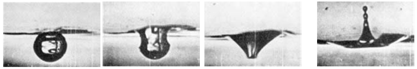Figure 13. Photographs by Blanchard (1963) of a bubble breaking through a free surface. Reproduced with permission of the author (Christopher 2005)

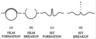Figure 14. Stages of a bubble breaking through a free surface

In both the industrial and oceanic processes, a key question is the range of droplet sizes that will almost immediately fall back into the liquid pool and, on the other hand, the range of droplet sizes that will be carried high into the atmosphere or cover gas. In the ocean, this significant transport above the water surface occurs as a result of turbulent mixing. In the industrial context of a liquid-fluidized bed, the upward transport is often the result of a sufficiently large upward gas flux whose velocity in the cover space exceeds the settling velocity of the droplet (Azbel and Liapis, 1983).

4. Flow Patterns

Bubbly flows are frequently encountered in chemical engineering. Much research on the hydrodynamics of these flows has been performed. Nevertheless, our understanding of the complex features found, for instance in a bubble column is limited. During the last decade CFD as a research tool has opened the possibility to perform detailed studies. Various approaches have been followed, generally divided into Euler-Lagrange (E-L) (Lapin and LuKbbert 1994, Devanathan et. al. 1995, Delnoij et. al. 1997, Hassan 2002, 2003, 2006, 2011, 2012, 2013, Hassan and Tamer 2006, Abdulmouti, et. al. 2000, Hassan et. al. 1997, 1998, 1999- No. 1, 1999- No. 2 and 2001, Hassan and Esam 2013) and Euler-Euler (E-E) based models (e.g. Grienberger and Hofmann 1992, Ranade 1992, Jakobsen and Torvik, 1992, Jakobsen 1993, Celik and Wang, 1994, Sokolichin and Eigenberger, 1994, Grevskott, Sannaes, Dudukovic, Hjarbo and Svendsen 1996). In the E-L Formulation a large number of particle trajectories is calculated using a previously computed liquid flow field, in which the interaction with the particles serves as a source in the momentum equation. In the E-E representation, the two phases are treated as interpenetrating fluids, represented by two sets of mass and momentum balances. Both approaches have been used to study the behavior of bubble columns. However, most of the simulations are not accompanied by experimental validation, mainly due to a lack of experimental data caused by the difficulties encountered when performing detailed hydrodynamic experiments. The bubble plume experiment of (Becker Sokolichin and Eigenberger 1994) has drawn quite some attention.

In general, bubble flow is defined as a Two-phase Flow where small bubbles are dispersed or suspended as discrete substances in a liquid continuum. Typical features of this flow are moving and deformable interfaces of bubbles in time and space domains and complex interactions between the interfaces, and also between the bubbles and the liquid flow. In general and according to the magnitude of these interactions, bubble flow is classified into four different flow regimes: i.e., ideally-separated bubble flow; interacting bubble flow; churn turbulent bubble flow; and clustered bubble flow, as shown in Figure 15. (Kataoka 1995).

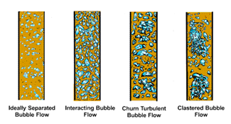Figure 15. Bubble flow regimes in vertical pipe flow

In ideally-separated bubble flow, the bubbles do not interact with each other directly or indirectly. The bubbles thus behave like single bubbles. In interacting bubble flow, bubble number density becomes so large that the bubbles begin to interact with each other directly or indirectly due to collisions or the effects of wakes caused by other bubbles. With a further increase in bubble number density, the bubbles tend to coalesce to form so-called cap bubbles, and the flow changes to churn turbulent bubble flow. The flow contains cap bubbles formed in this way and also smaller bubbles; it is highly agitated due to the interactions between bubble motions and turbulent flow. The large bubbles occasionally form clustering of bubbles, as shown in Figure 15, and they behave like a single gas slug. After a certain travel, they sometimes coalesce to form a gas slug and sometimes, they separate into individual bubbles. This flow regime is thus a transition from bubble flow to slug or churn flow. Quantitative criteria for the transitions from ideally-separated to interacting bubble flow, and from interacting bubble flow to churn turbulent bubble flow are roughly 0.01 and 0.06 in void fraction, respectively. Detailed discussions of single bubble behavior are given by (Wallis 1969).

Bubble flow is characterized by phase distribution phenomena, which exhibit different lateral void fraction profiles, depending on the volumetric flow rate of gas and liquid phases. Typical lateral void distribution patterns are given in Figure 16, representing wall void peaking, core void peaking and intermediate void peaking. For given flows of the two-phases in a given channel, the lateral void profile can take more or less of these forms. Figure 17 summarizes the trends of these void distribution patterns observed in vertically upward air-water in pipes using conventional types of bubble generators.

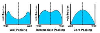Figure 16. Typical lateral void faction distribution patterns

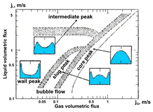Figure 17. Lateral void distribution patterns map for air-water flow in vertical pipes obtained by (Serizawa and Kataoka 1988)

4.1. Definition and Importance of Flow Patterns

In describing the configurations taken up by gas and liquid flowing together, researchers have used a very large number of names. Some of these are alternative names for the same flow pattern, whilst others are subdivisions of more major groupings. Much of this confusion has arisen from the subjective way in which flow patterns are characterized.

Initially, identification of flow pattern was by visual observation of the flow in transparent tubes, and this remains the primary definition. Given the almost infinite number of possible shapes and states of subdivision of the phases, a large number of reported flow patterns were inevitable. However, the number of flow patterns used in any description should be limited if the descriptions are to be of practical use, and a small number of major patterns have been agreed, as described below (B.J. Azzopardi 2012).

However, the problem remains of assigning a given flow to one of the agreed patterns. In narrow tubes, at moderate fluid velocities, visual observation is reasonably reliable, but at high velocities it is difficult to see anything, and in wider tubes and the shell side of heat exchangers only the flow near the wall can be seen. Photographs with a high speed flash, or high speed video studies, can help to overcome the problem of high fluid velocities, although it may be noted that some steam-water studies at a top laboratory in the 1960s using flash photographs had to be analyzed by majority vote among a team of experts!

More objective methods have been suggested for flow pattern determination. An early example used measurements of time-varying cross-sectionally averaged void fraction (fraction of cross-section occupied by gas) at one cross-section in a pipe using, e.g., X-rays, and plotted the Probability Density Function (PDF) of these measurements. This is the frequency of occurrence of each value of void fraction. The significant differences in the PDF “signatures” of different flow patterns that have been reported provide a, possibly more objective, means of flow pattern identification. In these, bubbly flow gave a single peak at low void fractions, annular flow a single peak at high void fractions, and intermittent flow gave two peaks. Analysis of pressure fluctuations, or, electrical resistance techniques related to time-varying void fraction have been employed. Other approaches used more sophisticated statistical analyses of time varying data. These more objective techniques are becoming increasingly popular, although there can still be disagreements between different investigators (B.J. Azzopardi 2012).

The major flow patterns for vertical up- and down-flow, horizontal flow and flow at other inclinations are defined below.

4.2. Flow Regime Types and Characteristics

4.2.1. Vertical Flow in Pipes:

Systems in which a gaseous phase is dispersed throughout a liquid are commonly encountered in both nature and industry. Known as gas-liquid flows, these systems occur in situations as diverse as the bow wave of a ship to the cooling system in a nuclear power plant. The structure of a gas-liquid flow depends upon the relative flow-rates of the two phases, and, for flow in a vertical pipe, can be categorized into four regimes (Mudde 2005).

Here, four main patterns or flow regimes are usually considered:

(i) Bubbly Flow or homogeneous (or dispersed)

(ii) Slug Flow

(iii) Churn Flow or heterogeneous (or discrete)

(iv) Annular Flow

Some authors make the distinction between bubbly flow or homogeneous (or dispersed) and churn flow or even (churn-turbulent) or heterogeneous (or discrete).

In these different flow regimes, the interaction of the dispersed gas phase with the continuous liquid phase varies considerably. However, bubbly and churn-turbulent flow regimes are most frequently encountered as shown in Figures 18 and 19. Depending upon the operating conditions, these two regimes can be separated by a transition regime (Ashfaq and Muthanna 2007, Hassan 2002, 2003, 2006, 2011, 2012, 2013, Hassan and Tamer 2006, Abdulmouti, et. al. 2000, Hassan et. al. 1997, 1998, 1999- No. 1, 1999- No. 2 and 2001, Hassan and Esam 2013).

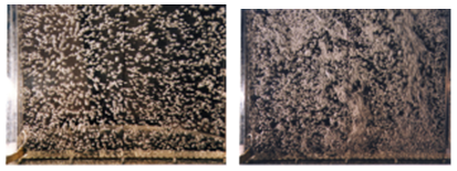Figure 18. Photographs of bubbly and churn-turbulent flow in 2-D column by (Ashfaq and Muthanna 2007)

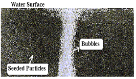Figure 19. Photographs of bubble plume with turbulent flow in 2-D column by (Hassan 2003)

Figures 20, 21, 22, 23, 24 and 25 show various flow regimes in bubble columns as illustrated by (Alexander 2011, B.J. Azzopardi 2012, Ashfaq and Muthanna 2007 among others).

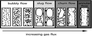Figure 20. The relation between gas flux and type of flow

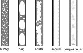Figure 21. Flow patterns in vertical up flow

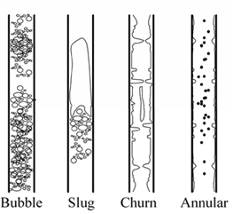Figure 22. Flow patterns in vertical up flow as (B.J. Azzopardi 2012)

Figure 23. Visual observations of four flow regimes encountered in bubble columns (Olmos et al., 2003)

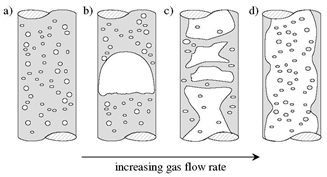Figure 24. Flow regimes for vertical gas-liquid flow as (Alexander 2011)

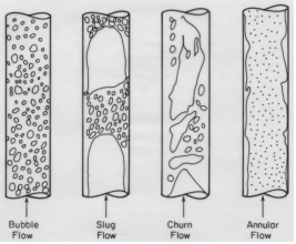Figure 25. Various flow regimes in bubble column reactors as (Ashfaq and Muthanna 2007)

(i) Bubbly flow: At low gas-fractions, the liquid is continuous and the gas exists as individual bubbles. Homogeneous flow occurs at low voidages, where the bubble size distribution (BSD) is narrow and there exists little interaction between bubbles, while with increasing gas-fraction the distribution broadens and bubble coalescence and break-up begin to occur. The boundary between homogeneous and heterogeneous bubbly flow is not well defined, however, bubbly flow to be treated as a single regime. Bubble flow consists of a continuous liquid phase with the gas phase is dispersed as bubbles within it. The bubbles travel with a complex motion within the flow, may be coalescing and are generally of non-uniform size. In some situations, they congregate mainly at the pipe centre, in others, near the pipe walls, and the wall-peaking and core peaking flows have sometimes been treated as sub-patterns of bubbly flow (Serizawa and Kataoka, 1988). At lower liquid velocities, the small bubbles must be generated either at the gas distributor or in the process of nucleate boiling, whereas at higher liquid velocities they can be formed by turbulent breakup of larger bubbles. Some workers treat these as two sub-patterns called discrete bubbly (or just bubbly) and dispersed bubbly flow respectively.

The homogeneous flow regime generally occurs at low to moderate superficial gas velocities. It is characterized by uniformly sized small bubbles traveling vertically with minor transverse and axial oscillations. There is practically no coalescence and break-up, hence there is a narrow bubble size distribution. The gas holdup distribution is radially uniform; therefore, bulk liquid circulation is insignificant. The size of the bubbles depends mainly on the nature of the gas distribution and the physical properties of the liquid (Ashfaq and Muthanna 2007).

(ii) Slug flow: As the gas-fraction increases, bubble coalescence becomes more prolific and the mean bubble size increases until slugs form which approach the diameter of the column. These slugs are periodic, and may exist with discrete bubbles still present in the intermediary. Some researchers have reported the occurrence of a slug flow regime only in small diameter columns.

The concentration of bubbles is not uniform but there are waves of drop concentration (void waves) in concentration which travel along the pipe Plug flow: This flow pattern, which in vertical systems is often referred to as slug flow, occurs when coalescence begins, and the bubble size tends towards that of the channel. Characteristic bullet-shaped bubbles, often called Taylor bubbles, flow up the pipe surrounded by a thin film of liquid. The liquid slug between the Taylor bubbles often contains a dispersion of smaller bubbles. Recent work has shown that this flow pattern does not occur in larger diameter pipes (150 and 200 mm), where there is a direct transition from bubble to churn.

(iii) Churn flow: In this regime neither phase is continuous; large irregular plugs of gas flow exist interspersed with slugs of liquid.

Heterogeneous flow occurs at high gas superficial velocities. Due to intense coalescence and break-up, small as well large bubbles appear in this regime, leading to wide bubble size distribution. The large bubbles churn through the liquid, and thus, it is called as churn-turbulent flow. The non-uniform gas holdup distribution across the radial direction causes bulk liquid circulation in this flow regime (Ashfaq and Muthanna 2007).

At higher velocities, the Taylor bubbles/liquid slugs in slug flow break down into an unstable pattern in which there is a churning or oscillatory motion of liquid in the tube. Churn flow with its characteristic oscillations is an important pattern, often covering a fairly wide range of gas flow rates. At the lower end of the range, it may be regarded as a breaking up of plug flow with occasional bridging across the tube by the liquid phase; whilst at the higher range of gas flow rates it may be considered as a degenerate form of annular flow with the direction of the film flow changing and very large waves (termed huge waves by some) being formed on the interface. In the latter range the term semi-annular flow has sometimes been used.

The Plug and Churn flow patterns, which both show large fluctuations in void fraction and pressure drop, are often grouped together as intermittent flow, particularly in shellside flows.

As one can see, homogeneous and heterogeneous flow regimes have entirely different hydrodynamic characteristics. Such different hydrodynamic characteristics result in different mixing as well as heat and mass transfer rates in these flow regimes. Therefore, the demarcation of flow regimes becomes an important task in the design and scale up of such reactors and has led to considerable research efforts which have resulted into various experimental methods and empirical, semi-empirical, and mechanistic models to identify flow regime transition (Ashfaq and Muthanna 2007).

The flow regime transition from bubbly to churn-turbulent flow or from churn-turbulent to slug flow depends simultaneously on parameters such as superficial gas velocity, column diameter, liquid and gas phase properties, and distributor design (Urseanu 2000). No flow regime map is available that covers a wide range of industrial conditions.

Bubble column applications can be classified based on their flow regimes. Most biochemical applications are performed in bubbly flow. Examples are cultivation of bacteria, cultivation of mold fungi, production of single cell protein, animal cell culture and treatment of sewage. In addition, other examples are hydro conversion of heavy oils and petroleum feedstocks, and coal hydrogenation. The churn turbulent flow regime is preferable for highly exothermic processes such as liquid phase methanol synthesis (LPMeOH), FT synthesis, and hydrogenation of MAC (Ashfaq and Muthanna 2007).

(iv) Annular flow: At high enough gas-flow rates only a film of liquid exists at the walls of the tube, with liquid droplets also entrained in the flow. Some authors describe other regimes at higher gas flow rates, including whispy annular flow (Hetsroni 1982).

Annular flow is characterized by liquid traveling as a film on the channel walls. Part of the liquid can also be carried as drops in the central gas core. In fact, for certain flow rates, the majority of the liquid travels as drops, leading to the term mist flow being applied to this flow pattern in some industries. However, only in heat transfer systems where walls can become too hot to be wetted is there flow with no liquid film, since in adiabatic systems a minimum film flow is needed before drops can be generated.

Interchange of liquid occurs between the film and the drops. Atomization of liquid to form drops does not occur over all of the film interface but from fast moving structures on the film interface which are usually termed disturbance waves. Under some circumstances, bubbles of gas can be entrained within the film. At very high liquid flow rates liquid concentrations in the gas core are so high that tendrils of liquid are observed instead of droplets. This is identified as wispy annular flow in some flow pattern maps.

In vertical down flow, flow patterns are very similar to up flow with bubble, plug, churn and annular flows being reported. However, these patterns occur over different ranges of flow rates. Thus, low gas and liquid rates, which would yield bubble or slug flow in vertical up flow, produce a falling film flow, which resembles annular flow.

4.2.2. Horizontal Flow in Pipes

When gravity acts perpendicularly to the tube axis separation of the phases can occur. This increases the possible number of flow patterns, as shown schematically in Figure 26.

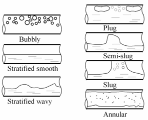Figure 26. Flow patterns in horizontal flow

Bubbly flow, like the equivalent pattern in vertical flow, consists of gas bubbles dispersed in a liquid continuum. However, except at very high liquid velocities when the intensity of the turbulence is enough to disperse the bubbles about the cross section, gravity tends to make bubbles accumulate in the upper part of the pipe as illustrated. In Stratified flow liquid flows in the lower part of the pipe with the gas above it. The interface is smooth. An increase of gas velocity causes waves to form on the interface of stratified flow to yield Wavy flows. Plug flow is characterized by bullet shaped gas bubbles as seen in vertical flow. However here they travel along the top of the pipe.

Slug flow, like plug flow, is intermittent. The gas bubbles are bigger whilst the liquid slugs contain many smaller bubbles. At large levels of aeration, they are called frothy surges or semi-slug, if the surges do not fill the pipe completely. However, this might be more correctly considered as part of wavy flow. A continuous gas core with a complete wall film characterizes annular flow. As in vertical flow, some of the liquid can be entrained as drops in the gas core. Gravity causes the film to be thicker on the bottom of the pipe but as the gas velocity is increased the film becomes circumferentially more uniform.

4.2.3. Pipes at Other Inclinations

Gas/liquid flow in inclined pipes is characterized by flow patterns similar to those described above for vertical and horizontal flows. For inclined up flow, the range of conditions occupied by slug-type flows, increases considerably starting at even small inclinations from the horizontal. For inclined down flow the range of conditions for slug-type flows diminish considerably.

4.3. Flow Pattern Maps

4.3.1. Vertical Flow in Pipes

Early work often represented the observed flow patterns on two-dimensional diagram in terms of system variables. The most common variables used are the liquid and gas superficial velocities (volumetric flow rate/cross sectional area of the pipe). Since variables other than the superficial velocities are known to affect the flow pattern, maps of this kind are specific to a particular combination of fluids and geometry. However, they are simple to use, and unlike the case of single-phase Newtonian flow where the single parameter of Reynolds number brings all flows together, it is indeed not easy to know exactly which other variables should be included. The reliable universal flow map should be produced.

The commonest way of constructing a flow map is to identify the flow pattern at a set of conditions covering the field, and then to sketch in boundary lines separating the different patterns. Because of problems in correctly identifying flow patterns, it often happens that a few experimental points lie on the wrong side of these lines, and the lines would be better regarded as transition zones, of indeterminate width. This should always be remembered when using maps on which only the boundary lines appear (B.J. Azzopardi 2012).

For vertical up flow, flow pattern maps based on superficial velocities have been published since the 1960's and are still being produced. Some workers have presented maps where the superficial velocities are modified by factors in the form of ratios of actual physical properties to standard values raised to different powers. A popular approach, which tries to incorporate some physical reality, is that of (Hewitt and Roberts 1969).

Vertical Down flow in Pipes, being less prevalent than up flow, has received less attention. Available studies are almost all for air/water in small diameter pipes published by (Barnea et al. 1982).

4.3.2. Horizontal Flow in Pipes

In horizontal flows the flow pattern map of (Baker 1954) still has great popularity. To its credit, it is simple and based on industrially relevant data (gas/condensate flows at high pressure in 5"-10" lines). Subsequent work has shown some of its transition boundaries to be poor. Much more popular is the composite map that illustrated by (Taitel and Dukler 1976).

For inclined flows (Spedding and Nguyen 1980, Gould 1972 and Mukerjee and Brill 1985), give maps for steep inclination. In addition, the (Taitel and Dukler 1976) approach can handle small deviations from the horizontal.

Information available on flows in horizontal pipes with non-Newtonian liquids and liquids with suspended solids has been collected by (Chhabra and Richardson 1985). They present specific flow pattern maps for both vertical and horizontal flows.

4.4. Two Phase Flow Pattern Observation and Map

Figure 27 of (Revellin 2005 and Revellin et al. 2006) showed the resulting laser signals for the respective flow patterns observed, actual images of selected flow patterns and schematic diagrams of the flow. As it is understood from the fact that intensity of light passing through any opaque medium will be more as compare to translucent medium thus voltage read for the first case more as compared to later case. In bubbly flow, the mean size of the bubbles shorter in length than patterns. The plots show the intensity of light (in negative voltage) versus time for the light incident on the diode and recorded by the data acquisition system. Even without any signal processing, it is possible to identify some flow patterns only by comparing the signals to the corresponding images; however, the corresponding videos were taken separately since its light source interfered with the diode light signals.

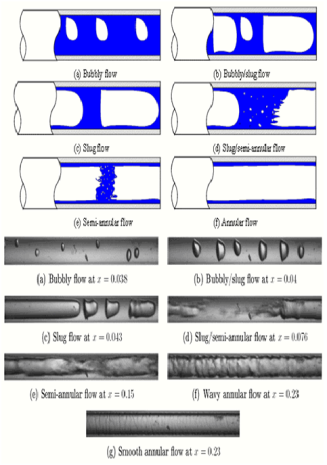Figure 27. Flow patterns and transitions observed by (Revellin 2006)

Processing the signals using the procedure described in (Revellin et al. 2006), it is possible to distinguish:

(i) the flow pattern,

(ii) the bubble frequency when they are present,

(iii) bubble velocity using a cross- correlation to find the delay time between the two signals,

(iv) the bubble length, and ( v ) indirectly the void fraction from the elongated bubble velocity.

(Revellin et al 2006) categorize the voltage into two threshold voltage two distinguish the presence and absence liquid and vapor in the flow. The minimum threshold voltage was -440mv below which the presence of liquid was detected and signals above -345mv justify the annular flow or an elongated bubble. Between this threshold nose and tail of bubble or frothy mix of liquid and vapor are present.

The above figure thus classifies these evaporating flow regimes as follows:

a) Isolated bubble regime: Initially at very low quality, the flow is usually found to be in bubbly flow regime which is characterized by discrete bubbles of vapor dispersed in a continuous liquid phase the channel diameter, slug flow (defined as bubbles longer than the channel diameter) and mixed bubble flows displaying both long and short bubbles and where the frequency of bubbles increases with increasing heat flux and thus vapor quality at a fixed mass velocity.

b) Slug flow: Slug flow defined as bubbles longer than the channel diameter. The nose of the bubble has characteristics of hemispherical cap and the vapor in the bubbles is separated from the wall by thin liquid film. In between the slug bubbles liquid is enclosed that separate the two slug bubbles.

c) Coalescing bubble régime: At slightly higher quality small bubbles may collapse this refers to slug flows that spans almost the entire cross section of the channel and thus frequency again decrease and then further increase and churn flows (the latter are long bubbles followed by aerated liquid slugs) but where some short bubbles may still exist, the flow for these condition is highly agitated resulting in a highly irregular interface.

d) Annular flow regime: This refers to both smooth annular flows with nearly no interfacial waves and wavy annular flow where interfacial waves are very evident. In this regime, the whole vapor is present at middle of pipe surrounded by annular liquid.

e) Dry out regime: after the annular flow regime, the vapor is dryout this is critical stage to be looked upon. This refers to the post- dryout region after passing through CHF at the critical vapor quality. In this stage vapor of extremely high quality exist and no trace of steam is left.

(Triplett et al. 1999) proposed a graphical map in terms of the superficial liquid velocity versus the superficial vapor velocity as shown in their paper, based on their flow pattern observations for air-water in a 1.1 mm horizontal glass channel (that is, essentially drawing in boundaries on the map). The flows were made using a mixer for the air and water upstream of the observation point. They also made observations in a 1.45 mm channel and in several small semi-triangular test sections using a strobe and digital camera for their observations. Also plotted on the map are the experimentally determined flow transitions for R- 134a of (Revellin et al. 2006) taken with the above described quantitative flow pattern detection technique.

These illustrate a significant difference in the transition locations, caused by the large difference in physical properties of air-water compared to R-134a. Hence, this points to the need of flow pattern transition prediction methods that incorporate the properties of the gas and liquid phases in order to generalize the map to work for other than the original fluid(s).

The topologies of multiphase flow patterns are illustrated in details in this section including explanation of flow regime maps:

4.4.1. Multiphase Flow Patterns

A particular type of geometric distribution of the components is called a flow pattern or flow regime and many of the names given to these flow patterns (such as annular flow or bubbly flow) are now quite standard. Usually the flow patterns are recognized by visual inspection, though other means such as analysis of the spectral content of the unsteady pressures or the fluctuations in the volume fraction have been devised for those circumstances in which visual information is difficult to obtain (Jones and Zuber, 1974).

For some of the simpler flows, such as those in vertical or horizontal pipes, a substantial number of investigations have been conducted to determine the dependence of the flow pattern on component volume fluxes, (jA, jB), on volume fraction and on the fluid properties such as density, viscosity, and surface tension. The results are often displayed in the form of a flow regime map that identifies the flow patterns occurring in various parts of a parameter space defined by the component flow rates. The flow rates used may be the volume fluxes, mass fluxes, momentum fluxes, or other similar quantities depending on the author. Perhaps the most widely used of these flow pattern maps is that for horizontal gas/liquid flow constructed by (Baker 1954). Summaries of these flow pattern studies and the various empirical laws extracted from them are a common feature in reviews of multiphase flow (see, for example, Wallis 1969 or Weisman 1983).

The boundaries between the various flow patterns in a flow pattern map occur because a regime becomes unstable as the boundary is approached and growth of this instability causes transition to another flow pattern. Like the laminar-to-turbulent transition in single phase flow, these multiphase transitions can be rather unpredictable since they may depend on otherwise minor features of the flow, such as the roughness of the walls or the entrance conditions. Hence, the flow pattern boundaries are not distinctive lines but more poorly defined transition zones. Nevertheless, there are other serious difficulties with most of the existing literature on flow pattern maps. One of the basic fluid mechanical problems is that these maps are often dimensional and therefore apply only to the specific pipe sizes and fluids employed by the investigator. A number of investigators (for example (Baker 1954, Schicht 1969 or Weisman and Kang 1981) have attempted to find generalized coordinates that would allow the map to cover different fluids and pipes of different sizes. However, such generalizations can only have limited value because several transitions are represented in most flow pattern maps and the corresponding instabilities are governed by different sets of fluid properties. For example, one transition might occur at a critical Weber number, whereas another boundary may be characterized by a particular Reynolds number. Hence, even for the simplest duct geometries, there exist no universal, dimensionless flow pattern maps that incorporate the full, parametric dependence of the boundaries on the fluid characteristics.

In single phase flow it is well established that an entrance length of 30 to 50 diameters is necessary to establish fully developed turbulent pipe flow.

The corresponding entrance lengths for multiphase flow patterns are less well established and it is quite possible that some of the reported experimental observations are for temporary or developing flow patterns. Moreover, the implicit assumption is often made that there exists a unique flow pattern for given fluids with given flow rates. We can see that even very simple models of multiphase flow can lead to conjugate states. Consequently, there may be several possible flow patterns whose occurrence may depend on the initial conditions, specifically on the manner in which the multiphase flow is generated (Christopher 2005).

4.4.2. Examples of Flow Regime Maps

Despite the issues and reservations discussed above, it is useful to provide some examples of flow regime maps along with the definitions that help distinguish the various regimes. The first examples were selected from the flows of mixtures of gas and liquid in horizontal and vertical tubes, mostly because these flows are of considerable industrial interest. However, many other types of flow regime maps could be used; examples are the flow regimes and those for granular flows.

(Hubbard and Dukler 1966, Wallis 1969, Weisman 1983) for example illustrated gas/liquid flows in horizontal pipes. Figure 28 shows the occurrence of different flow regimes for the flow of an air/water mixture in a horizontal, 5.1 cm diameter pipe where the regimes are distinguished visually using the definitions in figure 29. The experimentally observed transition regions are shown by the hatched areas in figure 28. Noting that in a mass flux map like this the ratio of the ordinate to the abscissa is X/(1−X) and therefore the mass quality, X, is known at every point in the map. There are many industrial processes in which the mass quality is a key flow parameter and therefore mass flux maps are often preferred. Other examples of flow regime maps for horizontal air/water flow (by different investigators) are shown in figures 30 and 31. These maps plot the volumetric fluxes rather than the mass fluxes but since the densities of the liquid and gas in these experiments are relatively constant, there is a rough equivalence. Note that in a volumetric flux map the ratio of the ordinate to the abscissa is β/(1 − β) and therefore the volumetric quality, β, is known at every point in the map (Christopher 2005).

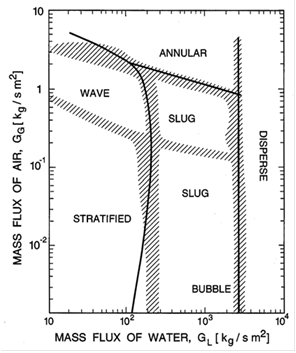Figure 28. Flow regime map for the horizontal flow of an air/water mixture in a 5.1 cm diameter pipe with flow regimes. Hatched regions are observed regime boundaries, lines are theoretical predictions. Adapted from (Weisman 1983)

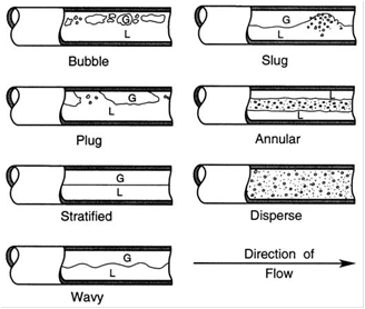Figure 29. Flow regimes for flow of air/water mixtures in a horizontal, 5.1 cm diameter pipe. Adapted from (Weisman 1983)

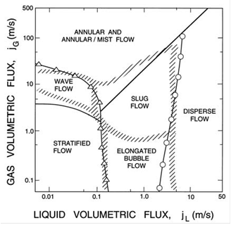Figure 30. A flow regime map for the flow of an air/water mixture in a horizontal, 2.5 cm diameter pipe at 25◦C and 1 bar. Solid lines and points are experimental observations of the transition conditions while the hatched zones represent theoretical predictions. From (Mandhane et al. 1974)

Figure 31 shows how the boundaries were observed to change with pipe diameter. Moreover, figures 28 and 31 appear to correspond fairly closely. Noting that both show well-mixed regimes occurring above some critical liquid flux and above some critical gas flux (Christopher 2005).

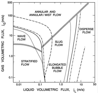Figure 31. showing changes in the flow regime boundaries for various pipe diameters: 1.25 cm (dotted lines), 2.5 cm (solid lines), 5 cm (dash-dot lines) and 30 cm (dashed lines). From (Mandhane et al. 1974)

4.4.3. Slurry Flow Regimes”

As a further example, consider the flow regimes manifest by slurry (solid/liquid mixture) flow in a horizontal pipeline. When the particles are small so that their settling velocity is much less than the turbulent mixing velocities in the fluid and when the volume fraction of solids is low or moderate, the flow will be well-mixed. This is termed the homogeneous flow regime (figure 32) and typically only occurs in practical slurry pipelines when all the particle sizes are of the order of tens of microns or less. When somewhat larger particles are present, vertical gradients will occur in the concentration and the regime is termed heterogeneous; moreover the larger particles will tend to sediment faster and so a vertical size gradient will also occur. The limit of this heterogeneous flow regime occurs when the particles form a packed bed in the bottom of the pipe. When a packed bed develops, the flow regime is known as a saltation flow. In a saltation flow, solid material may be transported in two ways, either because the bed moves en masse or because material in suspension above the bed is carried along by the suspending fluid (Christopher 2005).

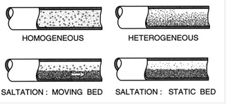Figure 32. Flow regimes for slurry flow in a horizontal pipeline

4.4.4. Vertical Pipe Flow”

When the pipe is oriented vertically, the regimes of gas/liquid flow are a little different as illustrated in figures 33 and 34 (see, for example, Hewitt and Hall Taylor 1970, Butterworth and Hewitt 1977, Hewit 1982, Whalley 1987). Another vertical flow regime map is shown in figure 35, which using momentum flux axes rather than volumetric or mass fluxes. Noting the wide range of flow rates in (Hewitt and Roberts 1969) flow regime map and the fact that they correlated both air/water data at atmospheric pressure and steam/water flow at high pressure (Christopher 2005).

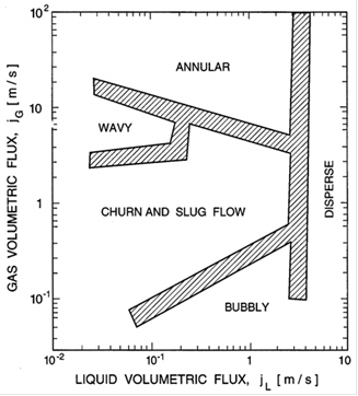Figure 33. A flow regime map for the flow of an air/water mixture in a vertical, 2.5 cm diameter pipe showing the experimentally observed transition regions hatched; the flow regimes are sketched in figure 32 Adapted from (Weisman 1983)

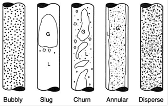Figure 34. Sketches of flow regimes for two-phase flow in a vertical pipe. Adapted from (Weisman 1983)

It should be added that flow regime information such as that presented in figure 35 appears to be valid both for flows that are not evolving with axial distance along the pipe and for flows, such as those in boiler tubes, in which the volume fraction is increasing with axial position. Figure 36 provides a sketch of the kind of evolution one might expect in a vertical boiler tube based on the flow regime maps given above.

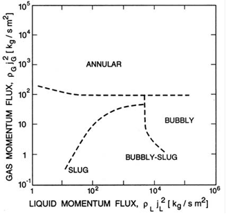Figure 35. The vertical flow regime map of (Hewitt and Roberts 1969) for flow in a 3.2 cm diameter tube, validated for both air/water flow at atmospheric pressure and steam/water flow at high pressure

4.4.5. Flow Pattern Classifications

One of the most fundamental characteristics of a multiphase flow pattern is the extent to which it involves global separation of the phases or components. At the two ends of the spectrum of separation characteristics are those flow patterns that are termed disperse and those that are termed separated. A disperse flow pattern is one in which one phase or component is widely distributed as drops, bubbles, or particles in the other continuous phase. On the other hand, a separated flow consists of separate, parallel streams of the two (or more) phases. Even within each of these limiting states, there are various degrees of component separation. The asymptotic limit of a disperse flow in which the disperse phase is distributed as an infinite number of infinitesimally small particles, bubbles, or drops is termed a homogeneous multiphase flow. This limit implies zero relative motion between the phases. However, there are many practical disperse flows, such as bubbly or mist flow in a pipe, in which the flow is quite disperse in that the particle size is much smaller than the pipe dimensions but in which the relative motion between the phases is significant (Christopher 2005).

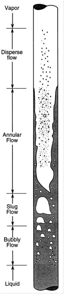Figure 36. The evolution of the steam/water flow in a vertical boiler tube

Within separated flows, there are similar gradations or degrees of phase separation. The low velocity flow of gas and liquid in a pipe that consists of two single phase streams can be designated a fully separated flow. On the other hand, most annular flows in a vertical pipe consist of a film of liquid on the walls and a central core of gas that contains a significant number of liquid droplets. These droplets are an important feature of annular flow and therefore the flow can only be regarded as partially separated.

As a summary, one of the basic characteristics of a flow pattern is the degree of separation of the phases into stream tubes of different concentrations. The degree of separation will, in turn, be determined by

(a) some balance between the fluid mechanical processes enhancing dispersion and those causing segregation,

or (b) the initial conditions or mechanism of generation of the multiphase flow,

or (c) some mix of both effects (Christopher 2005).

A second basic characteristic that is useful in classifying flow patterns is the level of intermittency in the volume fraction. Examples of intermittent flow patterns are slug flows in both vertical and horizontal pipe flows and the occurrence of interfacial waves in horizontal separated flow. The first separation characteristic was the degree of separation of the phases between stream tubes; this second, intermittency characteristic, can be viewed as the degree of periodic separation in the stream wise direction. The slugs or waves are kinematic or concentration waves (sometimes called continuity waves) (Christopher 2005).

4.4.6. Other Bubbly Flow Limits

As the volume fraction of gas or vapor is increased, a bubbly flow usually transitions to a mist flow, a metamorphosis that involves a switch in the continuous and disperse phases. However, there are several additional comments on this metamorphosis that need to be noted.

First, at very low flow rates, there are circumstances in which this transition does not occur at all and the bubbly flow becomes foam. Though the precise conditions necessary for this development are not clear, foams and their rheology have been the subject of considerable study, the reader may refer to the review by (Kraynik 1988 and Weaire and Hutzler 2001).

Second, though it is rarely mentioned, the reverse transition from mist flow to bubbly flow as the volume fraction decreases involves energy dissipation and an increase in pressure. This transition has been called a mixing shock (Witte 1969) and typically occurs when a droplet flow with significant relative motion transitions to a bubbly flow with negligible relative motion. (Witte 1969) has analyzed these mixing shocks and obtains expressions for the compression ratio across the mixing shock as a function of the upstream slip and Euler number (Christopher 2005).

5. The Wandering Phenomenon, Modeling and Measurements

Bubbly flows are encountered in many fields of engineering, pertaining to different spatial scales. At the small scale, they are found for instance in metallurgy in gas stirring of ladles, in nuclear devices, and chemical reactors; at extremely large scale, they take place in induced events of carbon dioxide sequestration, by which this compound is “injected” into deep seas. Bubble plumes in vessels present a particular feature, which is the “wandering” phenomenon. In general, simple terms, the flow swarms from side to side within the container. Some explanations for this behavior have been proposed, but they seem to be produced via instabilities of the flow enhanced by the presence of walls (Pfleger et al., 1999).

It is well known that a bubble plume often presents a wandering motion (Baines and Hamilton 1959, Fannelop et al. 1991, Fischer et al. 1994, Mudde et al. 1997b, Becker et al. 1999, Rensen and Roig 2001, Buwa and Ranade 2002, Joshi et al. 2002, Mudde 2005). The large amplitude wandering is a macro-scale turbulent process caused by the effects of the tank walls when the horizontal extent of the facility is not large in comparison with the plume diameter (Milgram 1983, Fannelop et al. 1991). An intermediate- and micro-scale turbulence process, with an energy distribution well represented by a Kolmogorov power spectrum, is superimposed on the wandering macro-scale turbulence process. These two processes produce turbulence at very different scales, thus contributing in different ways to the mixing in the tank.

In addition, bubble plumes in vessels present a particular feature, which is the “wandering” phenomenon. In general, simple terms, the flow swarms from side to side within the container. It seems to be produced via instabilities of the flow enhanced by the presence of walls (Pfleger et al., 1999).

(Fabian 2004) work is aimed at characterizing turbulence in bubble plumes undergoing a transient motion, a topic of primary importance in many environmental applications. Mathematical models for dilute mixtures, derived from the two-fluid model equations (multiphase flow theory), are initially presented. These models include diverse degrees of complexity, and they handle turbulence via a k-ε model and a Large-Eddy Simulation (LES) approach, in a consistent way. The models are implemented in a parallel code, which is then used to numerically simulate the dynamic behavior of bubble columns in three dimensions, using the LES approach. The results of high-resolution simulations show the presence of coherent structures whose distributions in space, and number, change with time. These structures are characterized in the paper via several indicators, connecting them with potential events of breakup of bubbles (Fabian 2004).

Furthermore, plume wandering has received scientific attention for about fifty years now. It has been observed not only in bubble plumes but also in single-phase, thermal plumes (Kotsovinos 1977). It is believed to be a buoyancy-driven instability enhanced by the presence of walls. It is worth pointing out that the phenomenon has nothing to do either neither with a sort of “Magnus effect”, (Johansen et. al. 1988) nor with “instabilities produced by excessive waves” (Castillejos and Brimacombe 1987). Typically, the bubbles swarm from side to side in the three dimensional space in a random manner. The motion has a quasi-period that depends on the airflow rate of the plume, and the aspect ratio of the container. (Delnoij et al. 1997) found experimentally that the frequency of the wandering motion increases with the aspect ratio (AR) for a constant airflow rate up to a value of AR ~ 4, after which a constant value for the frequency is attained. Larger airflow rates produce larger frequency values, i.e., smaller periods. These trends were confirmed by (Rensen and Roig 2001).

One set of measurements that has motivated much work during the last ten years is that performed by (Becker et al. 1994). Figure 37 shows pictures of a bubble plume undergoing wandering in a box of 0.5 m of width, 1.5 m of water depth, and 0.08 m of thickness perpendicular to the paper. They obtained velocity signals with Laser Doppler Anemometry (LDA), and presented time-averaged velocity fields.

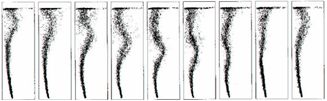Figure 37. Wandering motion in a bubble plume. Experiments by (Becker et al. 1994). Source: (Sokolichin and Eigenberger 1999)

Other measurements associated with wandering, in containers of different size and shape, were presented by (Mudde et al., 1999, Mudde and Van Den Akker 1999, Borchers et al., 1999, Becker et al. 1999, Lefebvre and Guy 1999, Pfleger et al. 1999, Rensen and Roig 2001, Brenn et al. 2002 and Buwa and Ranade 2002).

From the numerical point of view, the wandering phenomenon was the subject of several works, all of them employing finite differences. The state-of-the-art of the modeling of multiphase flows is such that there is no ample consensus on basic issues. (Tomiyama and Shimada 2001) stated that only a multi-group modeling of bubble columns (i.e., including processes of break-up and coalescence) guarantees the replication of wandering, whereas (Sokolichin and Eigenberger 1999) on the contrary, obtained wandering with a monodisperse model. Several researchers have also employed complex models to reproduce wandering, all of them based on the two-fluid model (TFM). This means that there is still a debate on how to model wandering and that, following (Loth 2000) the issue is still “what to model” rather than “how to model”.

It is intuitive to think that the numerical scheme is crucial in allowing for the replication of wandering. Very diffusive schemes could preclude the motion altogether. (Sokolichin et al. 2001) showed that solutions obtained with a very simple model (and without any turbulence closure!) using both an “upwind” scheme and a second-order TVD scheme were able to simulate wandering. However, eddies in the upwind solution did not show the level of detail in the length scales of the TVD solution. Sokolichin et al. also concluded that Lagrangean and Eulerian approaches offer similar results, provided that a large number of particles is used (they suggested more than100,000 particles). Later on, Sokolichin and Eigenberger reproduced wandering again with a simple model and the k- ε turbulence closure. In turn, (Deen et al. 2001) could not obtain wandering with the k-ε closure, but they could with a LES approach. On the other hand, (Mudde and Simonin 1999) stated that the addition of the lift force is mandatory to replicate wandering with the full TFM, a force that was ignored in many other simulations researches. Numerical simulations of the wandering phenomenon in bubble plumes obtained with a new comprehensive model was the focus of (Fabian et. al. 2004). The theoretical model was developed from the theory of multi-component fluids. The model was implemented in a finite-element, parallel platform. After a brief discussion about the theoretical/numerical model, the simulations of the wandering motion using the k-ε model was described and analyzed. This solution replicates wandering only for a relatively short period of time. The reasons for this fact are analyzed. Then, results obtained with the use of a Large-Eddy-Simulation (LES) approach were presented. These results notably mimic observations of bubble plume wandering without any restriction. Finally, the unsteady results of the LES approach was employed to perform a detailed analysis of turbulence in bubble plumes (Fabian et. al. 2004).

6. Two-Phase Slug Flow Measurements

Two-phase slug flow regime in a vertical pipe is characterized by large bullet-shaped bubbles, also called Taylor bubbles or gas slugs, which nearly occupy the entire cross section of the pipe. Between the gas slugs and the pipe wall flows a thin film of liquid. At the rear of the gas slugs there is a separated liquid region, the so-called bubble’s wake.

In daily life, this type of flow is encountered, for example, in a drinking straw that is being emptied too rapidly. In many industrial applications slug flow is present, for example, in the production and transportation of hydrocarbons in pipelines, in nuclear reactors during emergency core cooling, in boilers and in condensers (S. Nogueira et. al. 2003).

In a slugging column, with flowing gas and liquid, the flow field is extremely complex. In order to understand the hydrodynamics of such a complicated flow, the first step is to study the entire field around a single gas slug rising in stagnant liquid through a vertical pipe (S. Nogueira et. al. 2003).

(Campos and Guedes de Carvalho 1988) made a photographic study of the wake of isolated Taylor bubbles, and they identified three different types of wake regimes: laminar, transitional and turbulent, according to the value of N_f= (g^1/2 D^3/2 ρ)/µ. They presented empirical correlations for the length of the wake l_w as a function of N_f. The authors also suggested that, for long Taylor bubbles, the flow pattern in the wake is only determined by the velocity profile in the annular film. The flow in the annular region can be described as a falling film without shear stresses at the gas–liquid interface.

There are few studies in which PIV has been applied to slug flow, for example, (Polonsky et al. 1999 b) studied the motion of an isolated gas slug rising in a vertical pipe filled with water, for different liquid flow rates. They used an interlaced image technique to perform PIV measurements around the nose of the gas slug, which could not be used for higher liquid velocities, such those encountered in the annular film around the gas slug, where they had to use a streak length method. The shape of the gas slugs was determined separately, with an image-processing procedure applied to a sequence of video interlaced images (Polonsky et al. 1999a) of the bubble rising in water colored with a small amount of dye (0.001%) and illuminated by a 5-W laser.

(Van Hout et al. 2002) performed PIV measurements in slug flow for air–water systems, for stagnant water in the pipe. They determined the flow pattern around a single gas slug, and their results were in agreement with those of (Polonsky et al. 1999b) for the liquid film. They determined also, separately, the shape of the Taylor bubble, using the same procedure as (Polonsky et al. 1999a). In water, the permanent oscillations of the bubble bottom create no stationary field near the rear of the bubble. With the technique used, the authors had problems determining accurately the velocity field in this region.

(Bugg and Saad 2002) studied the flow around a Taylor bubble rising in a viscous solution and described the flow in a laminar wake. Since they determined the shape of the Taylor bubble by sketching the profile by hand, directly from the PIV image, they could not accurately define either the velocity field close to the interface or the bubble shape.

A recent technique of simultaneous particle image velocimetry (PIV) and pulsed shadow technique (PST) measurements, using only one black and white CCD camera, is successfully applied to the study of slug flow by (S. Nogueira et. al. 2003). The experimental facility and the operating principle are described. The technique is applied to study the liquid flow pattern around individual Taylor bubbles rising in an aqueous solution of glycerol with a dynamic viscosity of 113×10^-3 Pa s. With this technique the optical perturbations found in PIV measurements at the bubble interface are completely solved in the nose and in annular liquid film regions as well as in the rear of the bubble for cases in which the bottom is flat. However, for Taylor bubbles with concave oblate bottoms, some optical distortions appear and are discussed. This new technique that allows the simultaneous determination of the Taylor bubble’s shape and the flow field around the bubble, solving optical distortion effects that appear in two-phase PIV measurements, was successfully implemented. The technique consists of performing simultaneous PIV and pulsed shadow technique with a single black and white CCD camera. The measurements achieved a spatial resolution of 0.0022 tube diameters. The results obtained show high precision, solving completely the optical effects at the nose, in the annular film and in the rear of the bubble. The laminar close wake, rising up attached to the Taylor bubble, is clearly seen, the recirculation flow pattern is accurately determined and the wake boundary is defined. For the first time, the portion of the wake flow inside the concave bottom of the Taylor bubble is described. The optical distortion identified in this region, caused by the light crossing successive interfaces, is discussed. The results reported show high precision and are in agreement with theoretical and experimental published data (S. Nogueira et. al. 2003).

(Serizawa 2002, Feng and Serizawa 2001, Serizawa et al. 2002 and Serizawa 2004) listed several different flow patterns using air-water and steam-water flow in circular tubes of different µm size diameter: dispersed bubbly flow, slug flow, liquid ring flow, liquid lump flow, annular flow, skew (Yakitori) flow, frothy or whispy annular flow, rivulet flow and liquid droplet flow.

7. Micro Transition

7.1. Two Phase Boiling in Micro Channel

It is worth noting that what happens in microchannels is two-phase flow, which is quite different from single-phase flows in microchannels. Furthermore, many of the controlling phenomena and mechanisms change when passing from macrochannel two-phase flow and heat transfer to microchannels act. For example, surface tension (capillary) forces become much stronger as the channel size diminishes while gravitational forces are weakened. Therefore, it is usually not sensible to empirically refit macro scale methods to micro scale data since the underlying physics have substantially changed. This means that new dimensionless groups have come into play while the influence of others has disappeared (Sandhya 2007).

In recent years, the research in the field of single- and two-phase flow heat transfer at a micro scale level has been constantly increasing due to the rapid growth of the technology applications that require the transfer of high heat rates in a relatively small space and volume. (Suo and Griffith 1964) did the first study in micro Chanel of 1.03 and 1.60 mm diameter and observed three distinctive flow patterns: bubbly/slug, slug and annular flow. Their study covered heptane and water as the liquid phase, and helium and nitrogen as the gas phase. (Cornwell and Kew 1992) also noted three different flow patterns in rectangular channels (1.2 × 0.9 mm and 3.5 × 1.1 mm) for tests with R-113 and R-141b: isolated bubbles, confined bubbles, and slug/annular flow. He also postulated the concept of confinement number to note macro-to-micro transition.

Some authors as a further example, (Coleman and Garimella 1999) classified their observations into a total of 16 regimes subdivided into four main traditional groups (dispersed, intermittent, wavy and annular) that were then subdivided as follows: dispersed flow into 3 types of bubbly flow, intermittent flow into 4 types of slug and plug flow, wavy flow into 4 types of waves, and annular into 5 categories of annular films. Some very good photographs of the flow regimes are shown in their papers. (Yang and Shieh 2001) study on flow patterns of air-water and two-phase R-134a in small circular and was not able to predict different flow regimes for refrigerant flow. (Hetsroni et al. 2003) performed experiments for air-water and steam-water flow in parallel triangular microchannels and emphasized the discrepancy between flow patterns of air-water and steam-water flow.

An overview of the state-of-the-art of two-phase macro-to-micro scale transition criteria like bond number, confinement number and bubble departure diameter, two-phase flow patterns, void fractions and two-phase pressure drops in microchannels is described by (Sandhya 2007).

He addresses both experimental study for predicting two phase flow pattern regimes methods for micro channel and numerical expression to predict the frictional pressure drop across the micro channel. His objective of the investigation is to systematically study the gas liquid two-phase flow patterns, and pressure drop in capillaries with circular cross-sections (Sandhya 2007).

Numerous applications for micro scale flow boiling are emerging: high heat flux cooling of computer microprocessor chips and power electronics, precise cooling of micro-reactors, rapid and uniform cooling of LED displays, development of automotive evaporators with multi-port aluminum tubes, etc. All of these applications require thermal design methods that are accurate, reliable and robust (that is, methods that follow the trends of the data well and work for a multitude of fluids, channel sizes and shapes, pressures, flow rates, heat fluxes, etc.). Presently, the state-of-the-art is only partially able to fulfill such requirements in micro-channel heat sinks, channels are fabricated into the silicon chip (CPU), and coolant is pumped through them. The channels are designed with very large surface area which results in large heat transfers, further increased if two-phase flow cooling is applied (Sandhya 2007).

Rapid development of microfluidic devices has triggered the demand for a comprehensive understanding of the flow characteristics in microchannels to advance their design and process control. Micro scale devices can be fabricated using micromachining technologies and used for cooling microelectronic circuits, bioengineering applications, aerospace and micro heat pipes, among others. Some of these applications involve gas liquid two-phase flows in channels much less than 1 mm in diameter. The two-phase flow characteristics that need to be well understood include the two-phase flow regimes, void fraction and pressure drop.

From a point of view of applications, micro heat exchangers, micro cooling assemblies and thermal systems implementing such devices, referred to as micro-thermal-mechanical systems (MTMS) as opposed to micro-electronic-mechanical-systems (MEMS), are rapidly advancing to ever smaller sizes. These are used as micro cooling elements for electronic components, portable computer chips, radar and aerospace avionics components, and micro chemical reactors. Besides single-phase cooling applications, numerous two-phase (evaporation) cooling applications are being identified, for now being implemented without the benefit of thermal design methods for heat transfer and pressure drops (a difficult which is overcome by extensive testing). In fact, what can now be fabricated, either by micromachining of silicon wafers or micro extrusion of aluminum elements, has vastly outpaced what can be thermally modeled. In addition, while circular channels are the norm for macro scale evaporation processes, at the micro scale non-circular channels are more common. Thus, significant advances are required for the optimal development and operation of these devices (Sandhya 2007).

7.2. Macro to Micro Transition

In order to figure out different flow pattern for micro channel it is very necessary to know macro-to-micro transition dimension. Apparently, among the first to recognize macro-to-micro transition problem were (Mehendale and Jacobi 2000), who subdivided the macro-to-micro scale transition into four size classes (for convenience of discussion): micro scale (from 1 µm to 100 µm), mesoscale (from 100 µm to 1 mm), compact (from 1 mm to 6 mm) and macroscale (greater than 6 mm). (Kandlikar and Grande 2003) more recently recommended the following four classifications based on channel size of typical heat exchanger applications: nanochannels (<10 µm), microchannels (10 µm to 200 µm), minichannels (200 µm to 3 mm) and conventional channels (greater than 3 mm).

7.2.1. Evidence for Macro to Micro Transition

As mentioned in Engineering data book by Wolverine some evidence to support the existence of the macroto- micro scale transitions is first presented below and then methods proposed so far that attempt to identify these thresholds are described:

7.2.2. Flow Pattern Evidence for the Transition

On examining with high definition camera, 2.0, 0.790 and 0.509 mm horizontal channels Figure 38. It is found that as from macro-to-micro scale film becomes more and more uniform in shape. Interpreting images and many others available in the literature, one ascertains that stratified-wavy and fully stratified flows disappear (more or less completely) in small horizontal channels (Sandhya 2007).

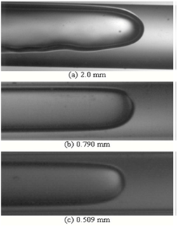Figure 38. The video image depict the dominant surface tension, in spite of buoyancy with diameter decrease (Remi et. al. 2006)

7.2.3. Void Fraction Evidence for Transition

Many scientists tried to figure out the variation of void fraction for transition from macro to microchannels and found a channels progressive deviation from the homogeneous void fraction law more and more sharply as the channel size was decreased.

7.2.4. Pressure Drop Evidence for Transition

The homogeneous model worked surprisingly well for flows that would fall in the slug and annular flow regimes, in fact much better than it usually does in comparison to similar macroscale pressure drop data. It is found that pressure drop data at the moment do not sustain the existence of a macro-to-micro scale transition in two-phase flow and thus requires a more detailed analysis than is feasible to better understand the counter-intuitive trend (Sandhya 2007).

8. Micro Bubble

Practical applications of micro bubble technology have recently become to attract people’s great concerns in wide variety of areas in advanced and conventional science and technologies, such as energy conversion and heat removal devices, diagnosis by ultrasound echo due to micro bubble collapse, drug delivery systems, cleaning and sterilization by shock waves due to the collapse of high pressure micro bubbles, production of ozone water, mining using physical absorption at gas-liquid interfaces, purification and improvement of oil-contaminated soil and polluted water by air supply (sea, lake, river etc), absorption of carbon dioxide gas, fish culture, etc. Here, the micro bubbles may be defined as the bubbles with diameters of the order of less than several tens microns, since these sizes of bubbles exhibit in fact somehow different behaviors from those observed with ordinary sized bubbles in their chemical and physical aspects.

What is a Micro Bubble and How Micro Bubble Behavior?

Micro bubbles with diameters smaller than several tens microns are supposed to have the following features:

(1) large interfacial area concentration for given void fraction.

(2) very low rise velocity-long residual time in liquid phase.

(3) very low possibility of bubble coalescence-good dispersion character and mixture homogeneity.

(4) dissolving character into liquid – bubble life (depending on the method of micro bubble generation).

(5) low electrical potential – good for physiological activation .

(6) physicochemical properties

(7) acoustic properties.

(8) fluid dynamic properties – reduction in skin friction, etc.

(9) others (Akimi et. al. 2003).

(Akimi et. al. 2003) concerns were focused on (1) what are bubble-turbulence eddy interactions? (2) what are bubble-bubble interactions ?

Based on a visual observation using a microscope, (Akimi et. al. 2003) found that micro bubbles behave like solid particles without significant shape deformation when they collide to each other (Fukami 2002). From this finding, (Akimi et. al. 2003) speculated on the micro bubble motions by numerical experiment, and came to a hypothetical bubble-bubble interaction force model which considers the effects of two major forces acting on two micro bubbles approaching to each other (Matsumoto et al. 2001).

Micro bubble technology has become to attract people’s concerns due to its wide potential in practical applications to a variety of advanced and conventional science and technologies. However, our knowledge of micro bubbles containing bubbly two-phase flow (which is limited) is to be broaden and expanded. A specially designed nozzle which generates high intensity micro air bubbles (mean diameter~ 40microns, number density more than 2×10⁵/cc) was developed by (Akimi et. al. 2003). Using this micro-bubble generator, as a first step, a measurement of two-phase frictional pressure drop, cross-sectional average void fraction and liquid velocity profiles were carried out. The measurement of local void fraction is underway. The range of average void fraction was up to 0.6 % which is enough to realize milky bubbly flow. The most exciting result was found is that the two-phase flow becomes laminarized by injecting such ultra small bubbles into the water flow. For 0.3~0.5% void fraction, laminar-turbulent transition occurred at Re=10,000~20,000. The cross sectional averaged void fraction does not follow a homogeneous flow model, and radial liquid velocity profile was a little bit flattened. The mechanism of flow laminarization and flow structures are now being pursued (Akimi et. al. 2003).

Moreover, microbubbles have considerable potential for the remediation of soils contaminated by organic compounds when used in conjunction with bioremediation technology (P. Jauregi and J. Varley 1999 and D. L. Michelsen 1991). They have advantages as an agent for stimulating biodegradation in a target site for the following reasons:

(i) microbubbles flow through porous media in a plug-flow manner, which can overcome like this the heterogeneity in soil (M. Lofti 1991 and T. A. Longe 1989, C. K. Mamun et. al. 2002 and J. Wan et. al. 2001).

(ii) they can enhance bacterial transport for the supply of pollutant-degraders (A. Jackson et. al. 1998).

(iii) deliver oxygen efficiently to a contaminated site for bioremediation (M. Lotfi 1990 and K. B. Jenkins et. al. 1993).

It was reported that a soil column spiked with p-xylene was treated successfully with an injection of oxygen-microbubbles (K. B. Jenkins et. al. 1993) and microbubbles containing pollutant-degraders enhanced the treatment efficacy of trichloroethylene (R. K. Rothmel 1998) or phenanthrene (Y. J. Choi et. al. 2007) in sand-packed columns.

A microbubble suspension is easily generated using a spinning disc type generator with a surfactant solution, as suggested by (F. Sebba 1985). Microbubbles, which are also referred to as colloidal gas aphrons (CGAs), have a spherical shape, are f 100 lm in size, and are stable when immersed in a liquid solution due to the encapsulated liquid film incorporated into their structure (F. Sebba 1971 and 1987). An understanding of the flow characteristics of microbubble suspensions in porous media is essential before they can be applied successfully to the subsurface for bioremediation purpose. In particular, the flow of gas in a microbubble suspension is of considerable interest because the gas phase serves as the primary medium for oxygen supply, which is crucial to aerobic bioremediation in the subsurface (J. Wan et. al. 2001 and K. B. Jenkins et. al. 1993).

Microbubble suspensions were generated as an oxygen carrier for aerobic biodegradation, and their flow characteristics in porous media were investigated by (Yong et. al. 2008). Commercial surfactants including sodium dodecyl sulfate (SDS), and dodecylethyldimethylammonium bromide (DEDAB), saponin (a natural surfactant), and collagen (a protein hydrolysate) were examined as base materials for generating microbubble suspensions. Among them, 26 CMC (critical micellar concentration) of SDS, DEDAB, and saponin developed microbubble suspensions with the highest gas hold-up and half-drainage time. Visualization of the flow patterns in sand showed that the microbubble suspensions were separated into a liquid and gas phase directly after injection, showing much faster movement of liquid phase flow. The gas front of the microbubble suspensions flowed in a plug-flow manner, particularly in cases of SDS and DEDAB. The experimental results from both homogeneous and heterogeneous cells confirmed that the microbubble flow could overcome the heterogeneity in porous media. However, the plug-flow characteristics and flow propagation of the microbubble suspensions to the low-permeability zone was accompanied by a large pressure drop, which needs to be considered for future field application (Yong et. al. 2008).

On the other hand, microbubble has useful characteristics such as very large specific surface area, very slow rising velocity, and good adsorbability. In (Koichi and Yasuyuki 2007) study, therefore, the microbubble flotation was utilized to separation of fine particles from water (Koichi and Yasuyuki 2007).

Microbubble flotation column

The flotation column which was made of steel has 125× 125 mm cross section, 1.00 m in height and a couple of wide sight glass windows. At the bottom, a high speed spiral liquid flow type microbubble generator (Nanoplanet Co; Ltd.: Type M2-LM) was set as gas distributor, in which gas was crushed to a lot of microbubbles by large shear stress due to the spiral liquid flow in the equipment (Koichi and Yasuyuki 2007).

Air was fed into liquid through the microbubble generator in 1.0 L/min. To make the spiral liquid flow in the microbubble generator, the liquid was circulated through it in 19.5 L/min using a pump (Koichi and Yasuyuki 2007).

Carbon particles and surfactants used

Fine carbon powder whose mean diameter is ca. 1 μm was used as the suspended particles. Tap waster tap water slightly added some kinds of surface active agents were used as continuous liquid phase (Koichi and Yasuyuki 2007).

The size distribution was measured using the photograph method. The mean diameter of the bubbles was 50 to 60 μm. The minimum and maximum diameter was 15 and 140 μm, respectively, which were independent from the kind of surfactants.

During 10 minutes bubbling, the fine carbon particles were removed from the liquid phase. The concentrated carbon particles were recovered in foam layer at the top of the flotation column.

As a result, by the microbubble flotation, fine carbon particle suspended in water was recovered. The removal mechanism was presented by the rates of adsorption to microbubble and remixing due to bubble breakage (Koichi and Yasuyuki 2007).

(Yoshiaki et. al. 2007) reports the current research status at NMRI toward practical application of microbubble, i.e. small air bubbles injected into the turbulent boundary layer, to ships as a drag reduction device. In order to obtain information on how much drag reduction is obtained in case microbubble is applied to a full scale ship, a 50m-long flat plate (1.0m width) was towed at 7m/sec, a typical cruising speed of a large tanker ship, in the 400m towing tank. Air was injected at the bottom, and not only the reduction of the total drag but also that of local skin friction were measured in a scale comparable to full scale (Kodama et al. 2004). Recently, in order to prevent injected air bubbles from escaping from the sides, end plates of 5cm height were attached on the two sides of the flat plate. A comparison of the measured local skin friction with and without the end plates was shown. The horizontal axis shows x_a, the downstream distance from the injection point located at 3m from the bow end, and the vertical axis shows the ratio of the local skin friction in the bubble case C_f to that of the non-bubble case C_f0 (Yoshiaki et. al. 2007).

The effect of the end plates is significant, and the skin friction reduction effect of approximately 50% by injected bubbles is well maintained up to the downstream end. This suggests that, in case microbubble is applied to a full scale ship, the skin friction reduction effect persists for a very long distance and, therefore, significant drag reduction is expected (Yoshiaki et. al. 2007).

(Yoshiaki et. al. 2007) also reports the propeller performance tests in bubbly flow, using two different sizes of propellers, both in non-cavitating and cavitating conditions. The two-dimensional wing section, whose shape agrees with that of the tested propeller at the 70% radial location, was also tested in bubbly flow. These results show that the propeller efficiency, or the lift-to-drag ratio of the wing section, is reduced in bubbly flow at small angles of attack, while it is much less affected at large angles of attack.

(Yoshiaki et. al. 2007) reports the two full scale experiments. In the first experiment, where the training ship "SEIUN-MARU", of length Lpp=105m, was used, the maximum drag reduction of 5% and net energy saving of 2% by microbubbles was obtained. In the second experiment, where the cement carrier "PACIFIC SEAGULL", of length Lpp=120m, was used, the air bubbles injected at the hull side did not go to the hull bottom sufficiently, and therefore, the maximum drag reduction was only 1%. In order to improve the drag reduction efficiency, various experimental studies mentioned above were carried out (Yoshiaki et. al. 2007).

Recently, microbubbles with the diameter of less than several μm are utilized in medical field such as contrast agent to ultrasound diagnostics and micro capsules for drag delivery systems. Characteristics of energy conversion of microbubbles are different due to its physical property. For instance, it’s known that kinetic energy by ultrasound is almost converted to thermal energy in case of Ar gas microbubble, on the other hand, it’s converted to acoustic energy in case of SF6 gas bubbles due to their specific heat ratio. It’s indicated that the appropriate inside gas of microbubbles for different applications are necessary. The microbubbles have been already used as contrast agents, the knowledge of the suitable combination of constituents of bubbles, which are gas and surfactant (or shell) for stable existence of bubbles in liquid, and generating techniques of microbubbles are very important to be established (Akiko et. al. 2007).

(Akiko et. al. 2007) proposed a simple microbubbles generator with diameter of several μm with different property of components of gas and surfactant by using a microchannel. In liquid-liquid two phase flow, former researchers realized to generate microcapsules or drops by using the shear flow in a microchannel (Thorsen et al. 2002, Anna et al., 2003), although in gas-liquid two phase flow, few research discussed the predominant factor to control bubble size (Garstecki et al. 2006). In a microchannel with T-junction, mono-dispersed microbubble can be generated. The smaller pressure difference was, the smaller bubble diameter became. And the faster liquid velocity was, the smaller bubble diameter became. When the bubble is generated at the T-junction in a main channel in their study, minimum diameter of generated bubbles is affected by the hydraulic equivalent diameter of gas injection. The minimum diameter attained in their study was 13.7 μm (Akiko et. al. 2007).

9. Homogeneous Turbulence Generation

Stationary turbulence was generated in a three-dimensional periodic box using a method that was suggested by (Eswaran and Pope 1988) and further developed by (Ruetsch and Maxey 1991, 1992 and Wang and Maxey 1993). The fluid was stirred by a random external force field throughout the domain, including the interior of the bubbles. This force (per unit mass) appeared as a body force in the Navier-Stokes equation.

As pointed out by (Wang and Maxey 1993), it is desirable that the force field should vary randomly in time so that the resulting turbulence can be spatially homogeneous. Earlier forcing schemes (e.g., Siggia, 1981, Squires and Eaton, 1991) used a stationary forcing function so that the turbulence statistics were spatially inhomogeneous. (Wang and Maxey 1993) used a stochastic forcing scheme that was suggested by (Eswaran and Pope 1988). The force was created by exciting the low-order Fourier modes using a Uhlenbeck-Ornstein (UO) stochastic process. The reader may refer to (Wang and Maxey1993 and Qian 2003) for the details.

In the experimental observations reported by (Risso and Fabre 1998), it was not feasible to determine the variations in the total surface area of a bubble. An advantage of numerical simulations is that this information is accessible and may be related to other items of interest such as the times at which a bubble breaks up. The measure of the bubble deformation based on its surface area, S*, as a function of the time measured in eddy turnover times for Runs 1 and 13. Figure 39 shows the mode of breakup for most of the bubbles that broke in the Simulations (D. QIAN et. al. 2006). No more than three child bubbles were ever observed in any of the simulations. However, as may be seen in the Figure, (Risso and Fabre 1998) found examples in which as many as 10 child bubbles formed. It seems possible that this difference is caused by the difference in the turbulent energy spectra in the simulations and the experiments. The energy spectrum in the simulations decreased more rapidly with wavenumber for wavelengths on the order of the bubble size than the corresponding spectrum in the experiments. Therefore, one would expect that there was less energy available to create the small-scale disturbances on the bubble surface that would be likely to create large numbers of child bubbles (D. QIAN et. al. 2006). Figure 39 shows images of the bubble just prior to and just after breakup for Run 4. The images in Figure 40 are not at equally spaced times; they were selected to show the typical behaviors of the bubbles. The bubble shapes are somewhat smoother than those shown by (Risso and Fabre 1998), which may be consistent with the notion that the energy spectrum for the simulated turbulence decreases more rapidly with wavenumber than the spectrum in the experiments (D. QIAN et. al. 2006).

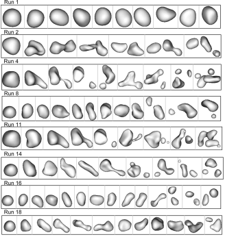Figure 39. Bubble breakup patterns

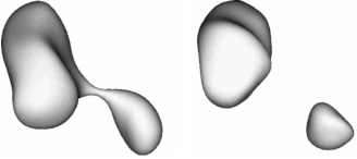Figure 40. Bubble breakup for Run 4

10. Conclusions

It is clear that the bubbly two-phase flow is an effective tool in many applications and can indeed contribute to various improvements since it is a key phenomenon to be studied and investigated. The purpose of studying the bubbly two-phase flow is the desire to develop its performance and its applications. The bubbly two-phase flow plays important and considerable roles in many engineering fields as materials, chemical, mechanical, modern industrial technologies, and in the environment. Hence, these engineering fields are expected to benefit from the improvement and development of the bubbly two-phase flow.

The present work demonstrates reviews and summarizes the major finding of previous research of the following points:

1) Bubbly two-phase flow characteristics, structures, behaviors and flow patterns.

2) Some important models and techniques to measure the two-phase bubbly flow parameters such as bubble motion, flow regime, bubble shape which play a considerable role in many engineering applications.

3) Some important applications of bubbly two-phase flow/bubble plume and its associated surface flow since it can contribute to improvements in various directions.