1. Introduction

The discovery of the Malagasy oil-fields is an asset in the economic development of the country. Indeed, due to the depletion of the currently exploited fields and the rarefaction of new field discovery, the Malagasy fields are going to open new economic opportunities for this fourth globally largest island. However, the control of a rational exploitation of a field means mastering various scientific techniques including the understanding of the dynamics of fluids in place. This goes to the sense where during the exploitation, fluids can enter and replace the fluids already in position, phases can appear or disappear, etc. However, the physical phenomena involved in an oil reservoir are complex. The understanding of these phenomena requires then the combination of physics, mathematics and computing [1, 2].

The “black-oil” model has been developed and used in several works for studying the dynamic behavior of fluids within oil reservoirs. Dehkordi and Manzari [3] used a multiscale finite volume method to multi-resolution coarse grid solvers for modeling a single phase incompressible flows. Mourzenko et al. [4] modeled a single phase and slightly compressible flow through a fracture porous media. The authors used a tetrahedral finite volume discretization for the rock matrix and triangular surface elements for fractures. Amir et al. [5] worked in modeling the flow of a single phase fluid in a porous medium with fractures using domain decomposition methods.

Douglas [6] surveyed a two-phase incompressible flow in porous media by using finite difference method. Douglas and Roberts [7] studied a single phase miscible displacement of one compressible fluid by another in a porous medium by using finite element method. Coutinho et al. [8] studied a black-oil model in an immiscible two-phase case such that gravity effects were not taken into account. Bell et al. [9] used a Godunov scheme of the first order and the second order for discretizing a two-phase black-oil model in one dimension. Miguel de la Cruz and Monsivais [10] studied a two phase flow model in porous media but the considered fluid was immiscible and incompressible; while using finite volume method for the discretization of equations. Using finite difference methods, Trangenstein and Bell [11] developed two-phase flow model incorporating compressibility and general mass transfer between phases. Chou and Li [12] developed a two-component model for the single-phase, miscible displacement of one compressible fluid by another in a reservoir.

Krogstad et al. [13] presented a three-phase black oil model. The multiscale mixed finite-element is used for the discretization of the equations. However, the model presented is related to immiscible flow and gravity is not taken into account. Geiger et al. [14] consider a three-phase black-oil model using a finite element/ finite volume scheme. In their study, they neglected the gravity forces and capillary forces. Abreu [15] presented a three-phase oil-water-gas model. However, this model does not take into account the compressibility of the flows and miscibility of component in phase. Lee et al. [16] has carried out the modeling of a three phase compressible flow in porous media. The authors used a multiscale finite volume scheme for the discretization of the equations of the model. However, the developed model was related to immiscible components. Hajibeygi and Jenny [17] applied a multiscale finite volume framework to model a mutilphase flow in porous media. Two models are considered in their works: the first model considers an incompressible flow and the second model considers a compressible multiphase flow. Nevertheless, in this work the miscibility is not taken into account. Lunati and Jenny [18] presented a model for compressible multiphase flow, wherein the multiscale finite volume method has been applied for the discretization of equations. However, their model is not related to a multicomponent system and the effect of gravity is not taken into account. Liu [19] considered two dimensional compressible miscible displacement flows in porous media. A finite difference scheme on grids with local refinement in time is constructed. The construction was done by use of a modified upwind approximation and a linear interpolation at the slave nodes.

Accordingly in the literature, there are rare works that study the three-phase compressible multicomponent flows using a finite volume scheme and take into account gravity and the miscibility of the lighter component in the oil phase.

The objective of the present investigation is to work out a numerical tool, capable of meeting the needs for understanding the dynamics of multiphase flows taking place within an oil reservoir. More precisely, while using the black-oil model, the compressibility, the miscibility of the lighter component in the oil phase, and the gravity were taken into account. The spatial discretization of flows was done by use of the cell-centered finite volume method. Implicit Euler scheme was used for the temporal discretization of equations. The studied model was coded on Matlab and the oil-field of Tsimiroro Madagascar was chosen for simulations.

Having the aforementioned numerical tool, it would be interesting to see the evolution of the model variables such as the pressure, the saturations of the present various phases in the reservoir and the accumulated flows of phases in the production well.

2. Methods

2.1. Simplifying Hypotheses

The “black-oil” model is considered as constituted by three fluid phases (oil, gas, and water) in each of them can be present the following three components: a lighter component (gas) which can be at the same time in the oil phase and in the gas phase, a heavier component which can only be in the oil phase, and a component water which can only be in the water phase [20]. The capillary pressures are assumed to be negligible [21, 13]. Accordingly, all the present phases in the reservoir have the same pressure. Moreover, the studied medium is considered as isotropic so that the components of the permeability tensor have the same values in all directions [10].

2.2. Mathematical Modeling

As there is a mass transfer between the oil and gas phases, mass conservation is not satisfied for these two phases. However, the total mass of each component is conserved. Besides, as the water phase is completely separated from the other phases and the component water is only present in the water phase, the mass conservation is well respected for this phase. Hence, the equations of the black-oil model can be formulated as follows [20].

Mass conservation related to the component water can be written as:

(1)

whereas for the heavier component, one can write:

(2)

and the lighter component is governed by:

(3)

where ρ_Go and ρ_Oo are the densities of the lighter and the heavier components in the oil phase respectively. Equation (3) implies that, the lighter component (gas) can be at the same time in the oil and the gas phases.

In equations (1) to (3), the velocity of each phase (α = w, o, g) is governed by the generalized Darcy’s law and can be calculated by the following relationship:

(4)

in which, denotes the tensor of the absolute permeabilities of the porous media, whereas g^→ denotes the gravity acceleration vector.

The system of equations (1) to (3) is completed by the following closing relationships:

- Conservation of pore volume (the sum of the saturations in a pore is equal to unity)

(5)

- Constraints on the capillary pressures (oil-water) p_cow and (gas-oil) p_cgo:

(6)

(7)

In order to ease the management of appearance and disappearance of a phase inside the reservoir, the formation volume factors of phases are introduced in the equations of mass conservation (1) to (3). For that purpose, the solubility of gas, denoted as R_so, has to be defined first as it permits to introduce the mass fraction of a component inside a phase. This parameter of solubility is defined as the volume of dissolved gas of the reservoir by unit volume of stored oil and is measured at standard conditions of pressure and temperature:

(8)

with

(9)

(10)

Equation (8) becomes then

(11)

The oil formation volume factor B_o is the ratio between the volume V_O that is measured at the reservoir conditions, and the volume V_Os of the component oil that is measured at standard conditions:

(12)

with

(13)

By reporting equations (9) and (13) into equation (12), this latter becomes:

(14)

From equations (11) and (14), the mass fractions of components oil C_Oo and gas C_Go in the oil phase are obtained respectively:

(15)

(16)

These mass fractions satisfy the closing relationship:

(17)

Then, it follows from equations (15) to (17) that:

(18)

The gas formation volume factor B_g is the ratio between the volume of gas phase measured at the reservoir conditions, and the volume of the component gas measured at standard conditions:

(19)

with

(20)

(21)

The expression of the density of free gas can be obtained from equations (19) to (21):

(22)

Similarly, the water formation volume factor B_w is defined by:

(23)

Finally, referring to relationships (18), (22) and (23) in equations (1) to (3) and taking into account Darcy's law for velocities, a new formulation of the black-oil model for components water, oil and gas respectively is obtained:

(24)

(25)

(26)

Equations (24) to (26) represent the equilibrium related to normal volume. Moreover, volumetric flow rates at normal volume are defined by:

(27)

(28)

(29)

where ρ_ws, ρ_os, and ρ_gs are constants which can be removed after substitution of equations (27) to (29) in equations (24) to (26).

The basic equations of the black-oil model are equations (1) to (3) and (24) to (26). The choice of the unknowns depends on the state of the reservoir which can be whether saturated or unsaturated. This case will be discussed in the section reserved for the numerical solution of the model equations.

The oil formation volume factor related to the unsaturated state depends on the bubble pressure p_b, the total pressure p within the reservoir and the oil compressibility c_o, and is formulated as follows:

(30)

in which B_ob is the oil formation volume factor at bubble pressure.

By use of an order one Taylor expansion, equation (30) can be rewritten as:

(31)

It is the same for the oil viscosity:

(32)

where μ_ob denotes the oil viscosity at bubble pressure p_b, while c_o being the oil isothermal compressibility and c_μ the oil viscosity compressibility.

It should be noted that in the saturated state, the bubble pressure is equal to that of the reservoir, and B_o and μ_o are only a function of pressure.

Equations (15), (17) and (18), permit to establish an expression of the mass fraction of the component gas in the oil C_Go in terms of the gas / oil relative solubility, and the densities of gas and of oil taken at standard conditions as follows:

(33)

Using equation (33), the ratio of solubility R_so can be expressed in terms of the mass fraction of the component gas in the oil and the densities of gas and oil taken at standard conditions:

(34)

The oil density can be a function of the pressure and the mass fraction of the component gas in the oil, that can be established from equations (14), (15) and (17). Indeed, by combining these three equations, the oil formation volume factor is given by:

(35)

While the oil formation volume factor being a function of pressure, equation (35) shows that the oil density is not only a function of pressure but it also depends on the mass fraction of the lighter component (gas) in the oil phase, as follows:

(36)

Thus, taking into account the expression of B_o given by equation (31), the oil density can be calculated by:

(37)

2.3. Thermodynamic Equilibrium

To study the thermodynamic equilibrium, the model proposed by Masson [22] is used. By Gibbs’ law, two-phase oil (o) - gas (g) equilibrium of a mixture of both lighter and heavier components, depends only on the pressure p when the temperature is assumed to be constant, which is the case in this work. This equilibrium is characterized by state laws of densities and and of viscosities and and the mass fraction of the lighter component in the oil phase (o). In the following section, barred symbol mean that the considered parameter is related to equilibrium state while unbarred one mean that there is no precision about the equilibrium state.

The thermodynamic of the black-oil system is given by the laws of and whose signs and variations are:

(38)

in which the apostrophe (') on any function indicates the derivative with respect to the pressure p of this function. It is worth noting that the equilibrium occurs when the reservoir pressure equals the bubble pressure. Thus, all symbols that are indexed by ob and that correspond to the state where the pressure is equal to the bubble pressure can be replaced, in the following, by barred symbols and vice versa.

Phase changes that may occur in the reservoir determine the transition from oil-gas-water (o-g-w) three-phase thermodynamic equilibrium state to oil-water (o-w) two-phase state, and are written in the following terms of unilateralism:

(39)

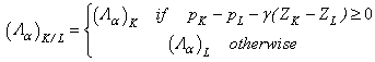
When the reservoir is in the oil-water two-phase state; in this case, oil phase is qualified as under saturated. On the other hand, if the reservoir is in the saturated state; this means that the three phases oil-gas-water coexist in the reservoir. The oil-gas two-phase state is observed when

The bubble pressure p_b is defined, similarly as done by Masson [22], by introducing the inverse function of that is here denoted by

(40)

with

(41)

where p_ref represents a reference pressure which is taken equal to the atmospheric pressure.

The gas phase appears, when the reservoir pressure drops below the bubble pressure. That is to say: p < p_b.

Disappearance of gas phase is indicated by a value of S_g that is inferior or equal to zero. In that case, one can write: S_g=0.

In the saturated state characterized by the existence of the three phases in the reservoir, the following condition is applied: p = p_b.

As it is the component gas that can completely dissolve in the oil phase, but there is no vaporization of the heavier component (oil) in the gas phase, the gas is the only component that can disappear and reappear according to the thermodynamic conditions previously presented by equation (39).

2.4. Numerical Procedures

2.4.1. Temporal and Spatial Discretization Methods

Temporal discretization is defined by the sequence tⁿ, n being a positive integer such that t⁰=0 and ∆tⁿ⁺¹=tⁿ⁺¹-tⁿ > 0; the superscript n implicitly means that the variable is considered at time tⁿ. An implicit Euler scheme is used for the time discretization.

A cell-centered finite volume scheme was used for spatial discretization. Indeed, the developed model is constituted by conservation equations. Since the finite volume schemes are conservative, they are better suited for solving the considered system of equations [23-24].

2.4.2. Boundary Conditions

All the borders of the reservoir are considered impervious. No flow either goes out or enters anywhere but places where wells are positioned. As depicted in Figure 1, four injection wells are placed in the four corners of the reservoir while a production well is placed in its center. A condition of pressure in each cell containing a well with perforation is imposed. While the injection of gas in the reservoir and in each cell containing an injection wells being the simulation object, gas saturation is considered equal to one.

Figure 1. Sketch of the reservoir with the four injection wells at the corners and the production well in the center

2.4.3. System of Discretized Equations

By applying the aforementioned discretization methods to the considered model, the following system of discretized equations is obtained:

(42)

(43)

(44)

in which

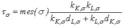
- is a singleton set whose element is the common edge σ between cells K and L (see Figure 2) and is equal to empty set otherwise.

- |K| is the volume of the cell K and Λ_α the mobility of the phase α (α = w, o, g) defined by:

(45)

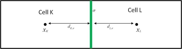Figure 2. Sketch of two neighboring cells K and L separated by a common edge σ

and it should be noted that an upstream off-center scheme was used to assess (Λ_α)_K/L as follows:

(46)

- τ_σ is the transmissibility between two neighboring cells K and L defined by:

(47)

- Q^α_lim,K (α=w,o,g) denotes boundary conditions in the cell K of α phase.

The system of discretized equations (42) to (44) is supplemented by the following equilibrium constraints:

(48)

The Newton-Raphson method was used for the linearization of the above nonlinear system of discretized equations (see Appendix) [25-28]. Afterward, the obtained linear system can be solved by classical methods of resolution of linear systems. In the present work, iterative Generalized Minimum Residual (GMRES) Method was used for this purpose.

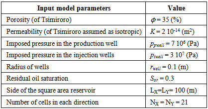
2.5. Data of Tsimiroro oil-field and Model Input Parameter Values for Simulations

It is worth noting that Tsimiroro is located approximately 125km from the west coast of Madagascar and the Best Estimate Original Oil in Place resulted in a Contingent Resource volume of 1.1 Billion barrels.

A log-log analysis of Tsimiroro wells was done to know the types of geological formations constituting the reservoir. Thus were obtained the reservoir petrophysical parameters including the porosity ϕ and permeability K of the site.

In addition to these petrophysical data, other model input parameter values that were used for simulations are also presented in Table 1.

Table 1. Input Model Parameter Values for Simulations

3. Results and Discussion

Results presented in the following figures are obtained by two-dimensionally (X,Y) simulating a three-phase oil-water-gas three components model whose lighter component may be simultaneously in the oil phase as well as in the gas phase. They show the evolution of the pressure, saturation and cumulative flow rate generated during the oil extraction.

Figures 3 and 4 show the pressure distribution in the reservoir per day and for five days of production. Observing isobars formed by these contours, it can clearly be understood how the pressure of the injection wells changes as when one approaches the producing well (in the middle). More precisely, this pressure is changing in two ways: it changes over both time and space. A spatial decay of pressure is observed while a temporal pressure increase occurs. The pressure imposed on the injection wells is higher than the pressure within the reservoir; the aforementioned spatial pressure decay that is observed following the fluid displacement front towards the center may be due to a pressure drop in the gas flow through the porous medium.

Moreover, the energy transferred by the gas to fluids that are in place (oil and water) justifies the temporal pressure increase. However, the pressure is still quite enough to push the oil to the production well and ease its drawing out. Indeed, the purpose of the gas injection in the reservoir is not only to increase the pressure, but also to make the oil less viscous to facilitate mobility for its extraction.

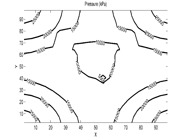Figure 3. Pressure for a production day

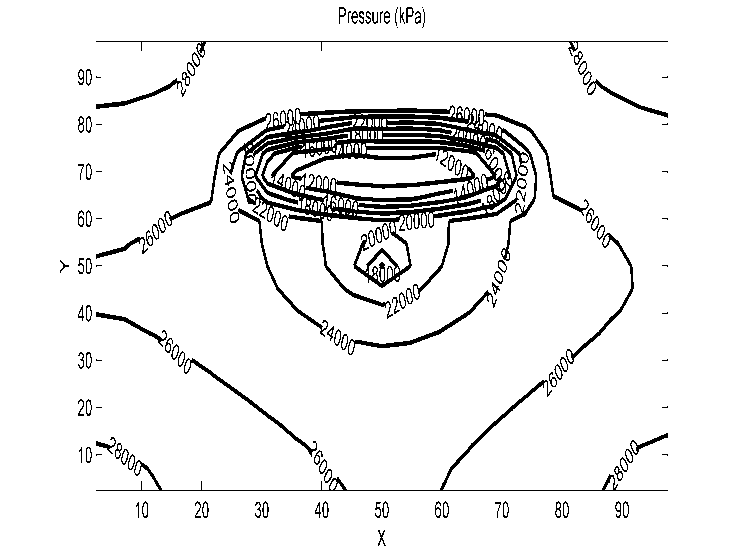Figure 4. Pressure for 5 days of production

Contours of saturations of various phases, that are present in the reservoir, are presented in Figures 5 to 10 which highlight the oil phase displacement front moving from the injection wells towards the production well. One can see that in areas of the reservoir where there is high gas saturation, there is low oil saturation. Indeed, while the injected gas being miscible in oil; it reduces the viscosity of the oil which makes it much more mobile. According to the values that can be seen on the contours of these graphs for the three phases in a given region of the reservoir, the closing law on saturation is well respected (conservation of pore volume). In addition, saturation of the water phase increases from the injection wells to the production well; this can be justified by the fact that in the reservoir there is water initially. Thus, during the gas injection, this water can be pushed by the gas to the production well. However, water being heavier than gas, this latter can be far more mobile than water, so that close to the production well, gas saturations are much higher than water saturations.

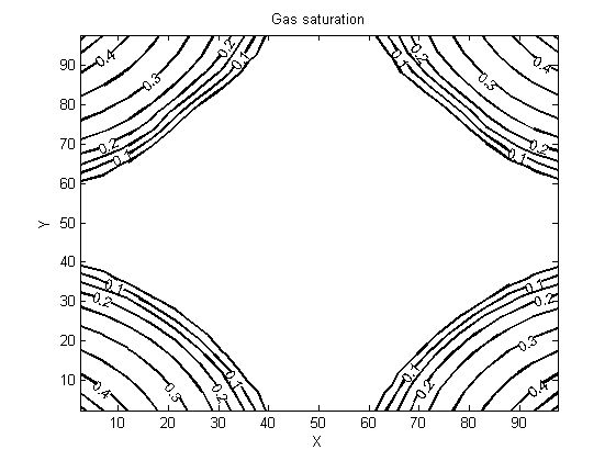Figure 5. Gas saturation for a production day

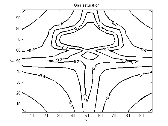Figure 6. Gas saturation for 5 days of production

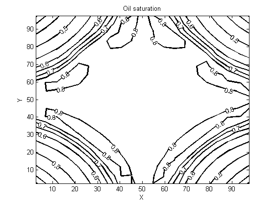Figure 7. Oil saturation for a production day

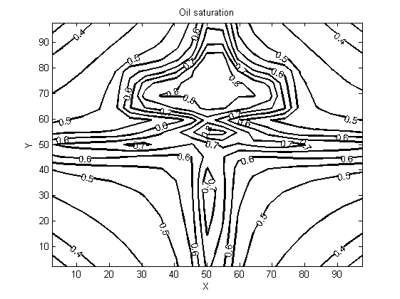Figure 8. Oil saturation for five days of production

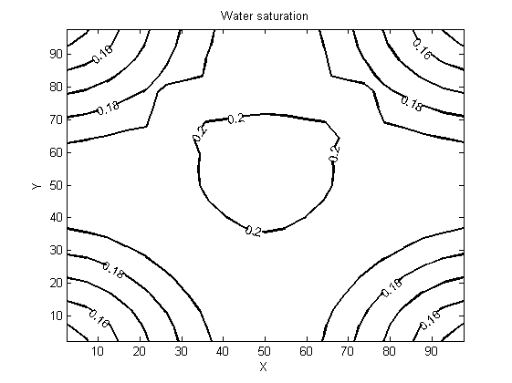Figure 9. Water saturation for a production day

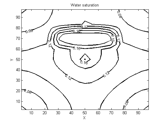Figure 10. Water saturation for five days of production

As can be seen from Figures 11 and 12 which show the variations of cumulative flow in the production well, a good amount of oil is produced. Such result conforms to the goal sought by the extraction process. The miscibility of the oil in the gas, combined with the fact that the oil is much lighter than the existing water, promotes such production. There is also a very low quantity of produced water which is lower compared to that of the produced gas, which itself is significantly less than that of produced oil. It can be justified by the fact that not only there may be an expansion of the gas during production, but the gas is also much lighter than water.

Figure 11. Cumulative flow in the production well for a production day

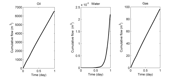Figure 12. Cumulative flow in the production well for 5 days of production

4. Conclusions

In the present work was studied a three-phase compressible multicomponent flow while using the black-oil model. More precisely, three components were considered: a lighter component (gas) which can be at the same time in the oil phase and in the gas phase, a heavier component which can only be in the oil phase, and a component water which can only be in the water phase.

The present study differs from other works [13-16] that have studied the compressible three-phase flows by the fact that it has taken into account both gravity and the miscibility of a lighter component in the oil phase, while using a finite volume scheme.

The considered model is complex as it comprises a nonlinear system of partial differential equations. A cell-centered finite volume discretization of the model has permitted to develop a Matlab code which has served to make numerical experiences on the extraction process of the oil field of Tsimiroro Madagascar.

It follows from simulation results that the code is able to predict the daily production operations (indicated by the cumulative flow), using gas as injected fluid. In addition, the mobility of the oil depends heavily on the gas saturation. When there is more gas somewhere in the reservoir, there is less oil. Besides, the conservation law of the pore volume is well respected.

As extension work, it would be interesting to consider the fact that the heavier component (oil) can evaporate into the gas-phase while using finite volume method. Another possibility of future work is also the thermal transfer study in which steam is injected into the reservoir. Indeed, such process is currently used by the company exploiting the Tsimiroro oil-field.

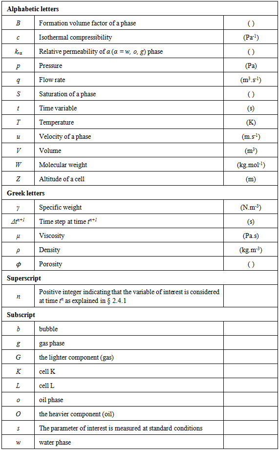
Nomenclature

Appendix

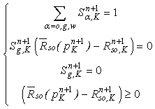
Management of appearance and disappearance of phase combined with Newton-Raphson method

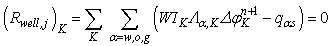
While interested readers being referred to [25-28] for more details, the principle of the Newton-Raphson method applied to the considered model is the following:

A vector R whose elements are the residuals in each cell is defined as:

(A1)

where N is the number of cells and m is the number of wells. In each cell i, one has:

(A2)

The expression of the residual in a cell K containing a well j (j=1,..., m) is defined by:

(A3)

in which, WI_K is the well productivity index of the cell K, and is the potential in the well of the cell K at time tⁿ⁺¹.

The Newton-Raphson algorithm requires the definition of the Jacobian matrix J such that:

(A4)

The submatrices of the matrix (A-4) are given by:

(A5)

Then, the following linear system is to be solved:

(A6)

In this equation, R^k and J^k are respectively the vector of residuals as defined by equation (A-1) and the Jacobian matrix at the Newton iteration k. Whereas δX^k+1 is the vector of unknown change. The unknown vector is updated at the Newton iteration by means of the following relationship:

(A7)

When a phase disappears, the saturation of this phase that is an unknown of the problem is replaced by the mass concentration of the lighter component. If all phases are present, the mass concentration is equal to the equilibrium concentration and is considered as a constant. Thus, a column vector of unknowns in each cell area containing the three primary unknowns of the problem is defined:

(A8)

in which, for each cell in the saturated state,

(A9)

and, for each cell in the unsaturated state,

(A10)

(A11)

where p_well,j is the pressure inside the well j.