1. Introduction

Over the last decades, bubble plumes (Buoyant plumes produced by a source of bubbles in a liquid medium) have had a number of applications in various engineering disciplines and fields, e.g. in industrial, materials, chemical, mechanical, civil, and environmental engineering applications such as chemical plants, nuclear power plants, naval engineering, the accumulation of surface slag in metal refining processes, the reduction of surfactants in chemical reactive processes, chemical reactions, waste treatment, gas mixing and resolution, heat and mass transfer, aeronautical and astronautical systems, biochemical reactors as well as distillation plants, etc (Hassan 2002, 2003, 2006, 2011, 2012, 2013, Hassan and Tamer 2006, Abdulmouti, et. al. 2000, Hassan et. al. 1997, 1998, 1999-　No. 1, 1999- No. 2 and 2001, Hassan and Esam 2013, Murai et. al. 2001, Abdel Aal et. al. 1966, Goosens and Smith 1975, Al Tawell and Landau 1977, Chesters et. al. 1980, Bankovic et. al. 1984, Sun and Faeth 1986a, b, Szekely et. al. 1988, Gross and Kuhlman 1992, Bulson 1968, A.W.G. de Vries 2001). Bubble plumes have been used with varying degrees of success. For instance, the following systems using bubble plumes were discussed in several literatures. (Taylor 1955) explained how bubble-breakwaters were operated by means of a surface jet produced by a bubble plume. He also demonstrated theoretically that the surface flow in the direction against the waves can break them. (Baines 1961) mentioned that the prevention of clean surface rivers or lakes from freezing over is possible using a bubble plume. (Baines and Leitch 1992) found that lines of bubble plumes have been used successfully to inhibit surface ice formation by bringing bottom water to the surface. They explained also that the most extensive application at that time was the destratification of reservoirs by mixing the lower-level water with the surface water. Denser water is lifted upward where the turbulence generated by the bubbles produces mixing with the lighter water. There is a similar process in metallurgical furnaces where the liquid metal or slag is heated from the top and hence is stratified. (Jones 1972) explained that bubble plumes can also contain oil slicks on water surfaces, and protect from underwater-explosion damage. (Marks and Cargo 1974) mentioned that bubble plumes were also useful for keeping swimming areas free from slow-moving objects such as sea nettles. Oil is very harmful to marine life and it is very difficult to clean the ocean from it (Hoults 1969). In addition, during an underwater oil-well blow-out, a plume of bubbles, oil droplets and sea water develops; the extent of the damage to marine life depends on whether all the oil rises to the surface or spreads out horizontally at some intermediate depth. Hence, nother interest in bubble plumes arises in the context of rectifying an oil-well blowout. Characteristically a lot of gas is emitted with the oil, and a plume develops due to the presence of bubbles formed by this gas (Topham 1974). (Mcdougall 1978) explained that the extent of damage caused by an oil-well blowout was strongly dependent on whether all the oil rises straight to the surface or some of it spreads out horizontally at some intermediate depth. (Kobus 1968 and McDougall 1978) made analytical studies on the vertical rising flow using experimental constants. (Shoichi et al 1982) measured two dimensional surface flow velocity profiles using hot wires as a basic tool for studying the prevention of oil diffusion with the help of a bubble plume.

Furthermore, bubble plumes have great application value in projects, such as alleviating the damage of wave to building structure, preventing the invasion of brine with air bubble curtain in estuary, controlling the stratification structure of reservoirs and lakes to improve water quality, enhancing oxygen for aquatic growth (Cheng Wen et al. 2008, Hassan 2002, 2003, 2006, 2011, 2012, 2013, Hassan and Tamer 2006, Abdulmouti, et. al. 2000, Hassan et. al. 1997, 1998, 1999-　No. 1, 1999- No. 2 and 2001, Hassan and Esam 2013). Therefore, the bubble plume has been a key issue in the current research field of fluid mechanics.

Moreover, bubble plumes have received considerable attention in the last four decades due to its large range of applications ranging from hydraulic engineering to high energy physics experiments. For example, they have been proposed as a means of containing surface-floating substances, such as oil from large oil spills in rivers and estuaries, they have been employed to augment convective heat and mass transfer rates in various chemical applications. Heat transfer through boiling is the preferred mode in most power plants and bubble-driven circulation systems are used in metal processing operations such as steel making, ladle metallurgy, and the secondary refining of aluminium and copper. Similarly, many natural processes involve bubbles. Bubble plumes have been employed for preventing icing in navigational waterways. One area of application that has received a great deal of recent attention is the use of bubble plumes as a desertification device, inducing mixing while introducing dissolved oxygen for improving water quality in lakes and reservoirs. As a mixing technique, the use of bubbles is attractive because it is very simple and cheap to operate. In particular, researcher interested in a recent application of bubbly fluids in the mitigation of cavitation damages in the Spallation Neutron Source (SNS) (Schladow 1992, Riemer et al. 2002 and Asghar and Gretar 1998).

Flows induced by a bubble plume are utilized in many industrial processes. The main features of this kind of flow are:

(1) A large scale circulation of the liquid phase can be generated in natural circulation systems like lakes, agitation tanks, etc.

(2) Strong rising flows can be induced by the pumping effect as in air-lifting pumps.

(3) High speed surface flows may be developed at the free surface, by which the density and the transportation of the surface floating substances can be controlled.

(4) A high turbulence energies can be produced in the two-phase region due to the strong local interaction between individual bubbles and the surrounding liquid flow. (Hassan 2002, 2003, 2006, 2011, 2012, 2013, Hassan and Tamer 2006, Abdulmouti, et. al. 2000, Hassan et. al. 1997, 1998, 1999-　No. 1, 1999- No. 2 and 2001, Hassan and Esam 2013, Murai et. al. 1999, Murai et. al. 2001).

As a result, by applying the bubble plume, the following processes are expected to be improved:

a- The prevention of sea water pollution by heavy oil leakage from tankers. Moreover, the development of the technology to prevent the diffusion of the leaked oil or oil generated from oil sources in the sea.

b- The prevention of diffusion of organic or harmful substances on the sea surface, lake surfaces and river surfaces, and the forced collection of them using the surface flow.

c- The prevention of freezing over of the surfaces of seas and lakes winter season and preventing channel and harbor from being freezed in.

d- Damping of waves propagating on the harbors, sea, lakes and rivers (pneumatic breakwaters).

e- Accumulation of the surface slag in the metal refining process.

f- The reduction of surfactants in chemical reaction processes. Beyond that, removal of oxide films or floating impurities from the surface of the chemical reactors in order to maintain the performance of reactions.

g- Prevention of surface sloshing in furnaces. Beyond that, removal of oxide films or floating impurities from the surface of the metal refining furnaces in order to maintain their performance. (Fabian 2004, Kristian and Iver 2008, Hassan 2002, 2003, 2006, 2011, 2012, 2013, Hassan and Tamer 2006, Abdulmouti, et. al. 2000, Hassan et. al. 1997, 1998, 1999-　No. 1, 1999- No. 2 and 2001, Hassan and Esam 2013).

In our paper (part-I), the major finding of previous research of bubbly two-phase flow characteristic, behaviors and flow patterns were elucidated, reviewed and summarized. Besides, some techniques and the important models for the measurement of the dominated two-phase bubbly flow/ bubble plume parameters were demonstrated.

The motivation of the present work (part-II that is extended to part-I) is the dement to demonstrate, review and summarize the major finding of bubble flow research. The measurement techniques and numerical modelings for the dominated two-phase bubbly flow/ bubble plume parameters are discussed in details such as gas flow rate, bubble size, bubble velocity and void fraction which are considerably important and play an important role in operational safety, process control and reliability of continuum processes of many engineering applications. In addition, the turbulent bubbly flow structure and some important applications especially on bubbly two-phase flow/bubble plume and its associated surface flow were reviewed since it can contribute to improvements in various directions are presented.

2. Bubble Parameters (Measurements, Techniques and Models)

A two-phase flow is one of the most common flows in nature as well as in many applications especially industrial; it covers gas-solid, liquid-liquid, solid-liquid and gas-liquid flows. Among these, the gas-liquid flows can be encountered in wide variety of industrial applications including boilers, distillation towers, chemical reactors, oil pipelines, nuclear reactors, etc. The measurement of two-phase flow parameters such as flow regime, bubble size and shape, bubble velocity and void fraction is considerably important and plays an important role in operational safety, process control and reliability of continuum processes (Dong, F. et al., 2003, Hassan 2002, 2003, 2006, 2011, 2012, 2013, Hassan and Tamer 2006, Abdulmouti, et. al. 2000, Hassan et. al. 1997, 1998, 1999- No. 1, 1999- No. 2 and 2001, Hassan and Esam 2013). The important methods and models to measure these dominated parameters are discussed in this section.

Two-phase flows have received much attention in the past few decades due to its importance in the power and process industries, to name a few. Consequently, there is a continuous need to enhance knowledge of the parameters affecting two-phase flows in piping systems. Although a significant body of knowledge on two-phase flow was generated, available experimental data tend to be limited to two-phase flow in small diameter pipes.

In the analysis of two-phase flow thermal-hydraulics, various formulations such as the homogeneous flow model drift flux model, and two-fluid model have been proposed. The two-fluid model considers each phase separately, in terms of two sets of conservation equations which govern the balance of mass, momentum and energy of each phase, and accounts for interface exchange through additional interfacial terms in the governing equations. Because of its detailed treatment of phase interactions, the two-fluid model can be considered the most accurate. However, the accuracy of the two-fluid model, and thus its usefulness in applications, depends on accurate modeling of the interfacial transfer terms. The Interfacial Area Concentration (IAC) is the main parameter in the interface exchange formulation and its importance can explicitly be seen in the basic conservation equations of the two-fluid model.

Many models and empirical relations have been proposed to formulate the IAC in terms of flow parameters such as gas and liquid superficial velocities, void fraction and pressure drop. However, available models are based on limited data for flows in small diameter pipes. The validity of these models for use in large-diameter pipes have not yet been determined (Ihab 1999).

Two-phase flow structure of an air-water, bubbly, upward, cocurrent flow in a large diameter pipe, 20 cm, was investigated experimentally by (Ihab 1999). Local flow parameters such as void fraction, bubble velocity, bubble diameter and interfacial area concentration were measured using a dual fiber optic probe. A well calibrated air-water testing loop was used to conduct the experimental work. A computerized data acquisition system was used to analyze the probe output signals and so measure the different flow parameters. The local time-averaged bubble diameter was measured using a direct averaging method and Uga's statistical method. The interfacial area concentration was measured using two methods; the bubble diameter-based method and the direct method proposed by (Kataoka et al. 1985). Whereas, void fraction is one of the most important parameter to characterize the hydrodynamic behavior of two phase dispersion system in a bubble column. The void fraction is a dimensionless quantity and is often termed as “holdup or fraction” in two-phase flows. It is defined as the ratio of the volume of that phase to the total volume of the pipe (Corneliussen, S. Et al., 2005) or can be defined as the fraction occupied by the gas phase in the total volume of a two- or three-phase mixture in a bubble column (Tang, C., 2006).

Results of the tests were compared with available data obtained for flow in small diameter pipes under the same flow conditions. Also, selected existing correlations based on data from small diameter pipe flows were applied to the data to check their applicability to flows in large diameter pipes. The results indicated the following under the same flow conditions:

1) Local void fraction ranging from 2.3 to 17.75 % and area-averaged void fraction ranging from 3.44 to 12.7 % were detected depending on the test conditions and radial position. Increasing the water superficial velocity at constant gas flow rate decreases the void fraction, and the bubble frequency, while it increases the bubble velocity. Any change in gas or water flow rates significantly affect the core values of these three parameters and slightly affect the near-the-wall values. The same effects were observed by increasing the air velocity at constant water velocity. The void fraction profiles are in good agreement with other profiles previously such as (Stankovic 1992) obtained under the same test conditions in small diameter pipes except for the saddle-type profile, which is frequently encountered in small diameter pipes under low area-averaged void fraction conditions.

2) The bubble diameter profiles were almost flat with a uniform distribution within the core region with increase in value near the wall. The two methods used to measure the bubble diameter, direct average method and Uga's statistical method, were in good agreement. The bubble diameter was generally insensitive to changing the flow rate, however, it increased with increasing the air velocity at constant water velocity. The bubble diameters were generally smaller than those obtained in small diameter pipes under the same flow conditions.

3) IAC profiles were obtained using bubble diameter-based method and the method of (Kaoaoka et al. 1985). The profiles were parabolic with lower value near the wall. Increasing the water flow rate under constant gas flow rate or decreasing gas flow rate under constant water flow rate, decreased the local IAC values with a more significant effect in the core zone. The work showed higher IAC values in large diameter pipes as compared with data obtained under the same flow conditions in small diameter pipes. Also, it showed higher area-averaged IAC than those predicted by applying the selected correlations. The agreement with available small-diameter pipe data and correlations improved at high gas and liquid flow rates (Ihab 1999).

In process industries, the measurement of void fraction is considerably important for sustainable operations. It largely affects the mass flow rate of gas and liquid in a two phase flow. The erroneous calculation of void fraction is inevitably be the cause of many industrial accidents such as loss of coolant accidents in reactors, sweet corrosions in sub-sea oil and gas pipelines and an in-efficient process control of chemical plants. The customary approach for two-phase flow measurement separates the two phases first and then measures the mixture as individual components. These methods are not favorable as they may result in the disruption of incessant industrial processes (Dong, F. et al., 2003; Ahmed, W.H., 2006).

Keeping in view the importance of measuring the void fraction, a non-invasive, experimental study was conducted by using Electrical Capacitance Tomography (ECT) technique and differential pressure (ΔP) technique on a concurrent vertical gas-liquid flow in a bubble column. A series of experiments were performed by regulating the flow rates of air and deionized water in a co-current bubble column to investigate the flow regime and void fraction. The flow characteristics were physically investigated by using visual instruments. In all the experiments air was used as a gas phase following the superficial velocity range of 0.00218 - 0.03 m/sec and deionized water as a liquid phase using the superficial velocity range of 0.00425 - 0.034 m/sec. The estimation of void fraction in a bubble column via ΔP method shows the influence of superficial gas velocity on void fraction as a linear function which agrees with the void fraction obtained from ECT measurements. The ECT measurement of void fraction also compared with photographic technique. It has been found from the analysis that the measurements generally follow the increasing trend of void fraction with an increase in superficial gas velocity (I. Ismail et. al. 2011). It is a common practice to use the normalized capacitance data for image reconstruction which is obtained from raw data measurements. The average void fraction of the ECT sensor was calculated using the normalized pixel values obtained from ECT images. The measurements obtained from these were in good agreement with (I. Ismail et. al. 2011) reference measurement obtained using ΔP. The estimation of void fraction using the differential pressure measurements was found to be increasing with increase in superficial gas velocity. The gas void fraction was initially a linear function of the superficial gas velocity, typical of the homogenous bubble flow regime. Both the methods follow the similar trend with respect to the increase in air flow rates. Their study has also estimated the volume void fraction using the photographic technique in a vertical upward column. It was also analyzed and validated from this technique that void fraction is a linear function of superficial gas velocity. On lower gas flow rate it shows a rapid increase in void fraction while, on higher gas flow rate the change in void fraction becomes steadily (I. Ismail et. al. 2011).

Whereas, two-phase flows represent a ubiquitous and extremely complicated phenomenon. Investigations of two-phase pipe flows are essential for various industrial applications that require reliable predictive quantitative solutions for design and maintenance. Accurate experimental data on the instantaneous distribution of both phases within the pipe are necessary for understanding the governing physical mechanisms in two-phase flow (Elena et. al. 2007).

(Elena et. al. 2007) study employs wire-mesh sensor as the measuring technique. This instrument enables experimental study of gas and liquid phase distribution in two-phase pipe flow. In addition, it allows determination of the instantaneous propagation velocities of the phase interface. (Prasser et al. 1998) were the first to apply the wire-mesh sensor for two-phase flow measurements. The instrument consists of three parallel wire layers perpendicular to the pipe axis. The wires in consecutive layers are directed normally to those in the previous layer, creating two meshes. The operation principle of the wire-mesh sensor is based on the difference in electrical conductivity of the two phases (water and air). The instrument can be seen as an intrusive tomograph that enables quantitative measurements of the cross sectional void fraction distribution. Being an intrusive instrument, wire mesh sensor is free of the inversion problems common to non-intrusive tomographs. The spatial resolution of the cross-sectional void fraction distribution is determined by the mesh geometry. The accuracy of the wire-mesh sensor was estimated against a technique used in previous investigation based on a borescope (Roitberg et al. 2006 a). Reasonable agreement between measurements results by both techniques was demonstrated by (Elena et. al. 2007).

Experiments are carried out in a 10 m long pipe with an internal diameter of 0.024 m. The pipe can be fixed at any angle of inclination. (Elena et. al. 2007) study deals with flow patterns observed in air-water downward pipe flow.

A novel algorithm for processing the wire-mesh sensor data was suggested by (Roitberg et al. 2006 b) to improve the spatial resolution of the sensor. The suggested algorithm is based on an approach used in computational fluid mechanics, such as the so-called volume of fluid (VOF) and takes into account the partial contribution of the neighboring junctions (Elena et. al. 2007).

Numerous parameters characterizing the interface shape variation for various operational conditions are obtained by (Elena et. al. 2007). In particular, the angle of the liquid film climbing along the cross sectional perimeter and interface shape fluctuations are studied. The 3D structure of the two-phase flow distribution within the pipe is obtained for stratified, slug and annular flow patterns. In the slug flow regime, the shapes of the bubble nose, liquid film and bubble tail are determined (Elena et. al. 2007).

Furthermore, void fraction and interfacial area are two key geometric parameters that accurately specify the phase interaction terms in the context of two-fluid models. The dynamic computation of the interfacial area concentration dispenses with the use of flow-regime dependent correlations or fixed morphology characterized by a single size scale. The model coefficients for the one group interfacial area transport equation (IATE) applicable to bubbly flows originally derived by (Kim et al. 2002) are revisited. A multi-objective optimization approach is pursued instead of an isolated parameter method. The goal of using the optimization method is to demonstrate the utility of such an approach (John et. al. 2007).

The nine flow conditions were originally considered by (Kim et al. 2002). These cases are classified as bubbly flow cases with respect to the flow regime map of Mishima and Ishii (1984); flow regime boundaries delineated through visualization experiments. This is significant because the double wire conductivity probe used in the experimental measurements of (Kim 1999) is not capable of characterizing two group interfacial area dynamics (John et. al. 2007).

The one group IAT models have six adjustable input parameters for the source and sink terms to be set by comparisons to experimental data: for the wake entrainment, C_WE; for the random collision, C_RC; for the turbulent impact, C_TI; a critical Weber number, We_cr; and constants approximating the normalized collision length scale, C, and the maximum void fraction, max α_max, in the random collision sink. The constants presented in (Kim et al. 2002) were derived by modeling the contributions of individual source and sink terms to the interfacial area concentration and arriving at values by matching runs with dominant mechanisms, i.e., isolating individual parameters. (John et. al. 2007).

In (John et. al. 2007) work, the test data from bubbly flow experimental conditions are considered and a multi-objective optimization approach is used to determine the six adjustable constants. To perform the optimization on the model constants, mode FRONTIER (ver. 3.2.0, ES.TEC.O srl, Treiste, Italy) is used to drive MATLAB (ver. 7.1, The MathWorks, Inc., Natick, MA) simulations of the one dimensional drift flux formulation of the problem. Objective functions are constructed to minimize the error between the computed and experimental interfacial area concentration across the range of bubbly flow conditions. Certain reasonable limits to the parameter space, e.g., to the critical Weber number, is applied as appropriate. The goal of this analysis is to regenerate the modeling constants using a different approach and show the usefulness of higher level analytic tools. Eventually, multi-objective optimization could be used for pointwise comparisons to experimental data with the one group IATE implemented in a two-fluid CFD code. The approach would relax some of the assumptions in the drift flux modeling related to the liquid velocity profile, but introduce additional complications related to the computation of the turbulent dissipation necessary in the turbulent impact and random collision sources (John et. al. 2007).

In fact, bubbly flows are complicated to simulate, because the internal geometry of the problem typically varies with time and the fluids involved can have very different material properties. Mathematically, bubbly flows are modeled using the Navier-Stokes equations, which can be approximated numerically using operator-splitting techniques. In these schemes, equations for the velocity and pressure are solved sequentially at each time step. In many popular operator-splitting methods, the pressure-correction is formulated implicitly, requiring the solution of a linear system at each time step. This system with a symmetric positive semi-definite (SPSD) coefficient matrix takes the form of a pressure Poisson equation with discontinuous coefficients (Bunner and Tryggvason 2002, Hua and Lou 2007, Jok 2009).

However, over the last 20 years, various methods have been developed for the simulation of the gas-liquid interface in bubbly flow. These methods can be divided into two main categories: “one” and “two” fluid methods. In one fluid methods, a single set of conservation equations is solved and the interface between the two fluids is tracked or captured. On the other hand, in two fluid methods, a set of conservation equations is solved for each phase and the interaction between the phases is given by some correlations. In the modeling of two-phase flows, one fluid methods are more widely used than two fluid methods. Focusing on one fluid methods, two types of approach are used to compute interfacial motion: interface tracking and interface capturing methods. The main difference between these methods is that interface tracking is Lagrangian while interface capturing is Eulerian (Bogdan et. al. 2010).

A fully 3D parallel and Cartesian level set method was coupled with the volume of fluid method within the commercial CFD code FLUENT by (Bogdan et. al. 2010). In this CLSVOF method, the level set function was used to compute the surface tension contribution to the Navier–Stokes equations more accurately than the VOF method by itself. The volume of fluid function was then used to capture the interface. By doing this, the two drawbacks of the LS and the VOF methods were overcame: the mass conservation problem of the LS method and the rather poor calculation of curvature and normal vector to the interface for the VOF method (Bogdan et. al. 2010). The level-set method is not only to improve the calculation of surface tension, but also to improve the surface reconstruction in VOF method, which is critical to the calculation of volume flux in the grid cell across the interface.

A re-initialization equation was solved after each time step for the level set function. This equation was discretized using a fifth order weighted essentially nonoscillatory (WENO) scheme for spatial derivatives and a first-order Euler explicit method for time integration. The method was implemented on both serial and parallel solvers. The coupling between LS and VOF was achieved by solving, at the and of each time step, an equation, which connects the volume fractions with the level set function.

The basic idea behind level set method is to consider a smooth continuous scalar function which is zero at the interface, positive in one phase and negative in the other phase. Usually, is initialized as the signed minimum distance function to the interface, so for the whole domain. Later on, when we need to solve the re-initialization equation, is true only at the interface. In case of an arbitrary initial interface, the re-initialization equation should be solved at the beginning of the calculation to ensure that at least near the interface the level set function is a signed distance. When the interface is advected by an external velocity field, the evolution of the level set function is given by (Bogdan et. al. 2010).

The static bubble simulation that performed by (Bogdan et. al. 2010) showed a reduction in the strength of the spurious currents around the bubble by approximately 51% using CLSVOF compared with VOF. This is explained by the fact that the level set function is a continuous function as opposed to the volume of fluid function and, thus, the surface tension force is discretized more accurately. A droplet deformation due to a vortex velocity field was also simulated by (Bogdan et. al. 2010). The interface position, after undergoing severe deformation, was recovered at the initial position with a very small perturbation for the coarsest grid and insignificantly for the finest grid.

For a series of bubbles rising in a stagnant fluid, (Bogdan et. al. 2010) achieved good agreement with the experimental data available from (Bhaga and Weber 1981) with a maximum relative error of approximately 16% using CLSVOF while with VOF the maximum relative error was approximately 19%. Using a 3D-axisymmetric domain a better accuracy with a maximum relative error of approximately 9% was achieved. A very good agreement was also obtained when (Bogdan et. al. 2010) compared the results obtained with their CLSVOF code with the experimental data of (Hnat and Buckmaster 1976). Although for the air-water sugar simulations the difference between CLSVOF and VOF was almost insignificant, for the air-water simulations CLSVOF performed better than VOF itself. Furthermore, vortex shedding was predicted to occur as expected with CLSVOF but not with VOF. Although the relative error for the bubble mean lateral displacement was rather large using CLSVOF compared with the experiments from literature, CLSVOF (bubble mean lateral displacement of 0.885 mm), generally, performs better than VOF (where the bubble mean lateral displacement of 1.7 mm is due to the shift of the bubble rectilinear path). The bubble rise velocities obtained with CLSVOF and VOF were comparable with the experimental values with slightly better accuracy achieved with the CLSVOF method. Using dimensionless analysis and moving wall approach, air bubbles of 2 mm, 3 mm, and 4 mm rising in still water were also computed using CLSVOF. The obtained bubble rise velocity compared well with experimental results from literature (Bogdan et. al. 2010).

In addition, models are developed to describe the gross behavior of air-bubble plumes generated by point and line sources of air-bubbles released in stagnant water bodies of uniform density. The models predict plume width, velocities, and induced flow rates as a function of elevation above the source. The analysis is confined to the plume mechanics and does not include the horizontal flow created at the surface by the plume. An integral similarity approach, similar to that used for single-phase buoyant plumes, is employed. Governing equations are found by applying conservation of mass, momentum, and buoyancy. The compressibility of the air and the differential velocity between the rising air bubbles and water are introduced in the buoyancy flux equation. Generalized solutions to the normalized governing equations are presented for both point and line sources of air-bubbles (Klas and John 1970).

The similarity between the air-bubble plume and a single phase buoyant plume was first pointed out by (Taylor 1955) in a discussion of pneumatic breakwaters. He noted that the similarity existed only if the air bubbles were so small that their rise velocity relative to the induced plume velocity was negligible. This restriction and attempts to account for the existence of such relative motion was relaxed. (Bulson 1962) found semi-empirical relations for the maximum velocity and thickness of the layer of horizontal surface flow. (Sjoberg 1967 and Kobus 1968) have investigated, both experimentally and analytically, air-bubble plumes using the concepts of jet and plume mixing (Klas and John 1970).

As air is discharged into water from a nozzle it breaks up into bubbles of discrete size. A study of the formation of gas bubbles in liquids has been reported by (Davidson and Schuler 1960). The rise and motion of individual gas bubbles in liquids have been investigated in many studies, and for example, (Haberman and Morton 1954), have reported on a comprehensive study on the rise velocity of single air bubbles in still water.

The analyses and generalized solutions for the cases of point source and line source air-bubble plumes provide predictions of the gross hydrodynamic features of such systems. These features are the velocity, width, and volume flux as a function of distance above the source. Comparisons of the analyses with large-scale experimental results indicated good agreement and yielded values for the lateral spreading ratio parameter and the entrainment coefficients. Application of the results requires that, in addition to the air discharge rate and description of the receiving water environment, an estimate of the bubble rise velocity in still water is provided. Such estimates are available as a function of bubble size (Haberman and Morton 1954 and Klas and John 1970).

Air-bubble plumes have had a variety of applications in coastal waters including the inhibition of ice formation, pneumatic breakwaters, barriers to minimize salt water intrusion in locks, containment of oil spills, and mixing for water quality control.

The discharge of air-bubbles into water creates a turbulent plume of an upward rising mixture of air and water by reducing the local bulk density of water. The rising plume entrains water from over the depth until it reaches the surface region, where as shown in Figure 1 and 2, a horizontal current is created. This study is restricted to the region below the influence of horizontal flow, and provides predictions of the flow delivered to this surface region. Experimental evidence indicates that the region of horizontal flow is approximately 0.25 of the water depth above a line source and somewhat less for a point source (Klas and John 1970).

A new measurement technique for multi-phase flow was proposed by (Hideki et. al. 2004) to measure two kinds of phases at the same place and the time, Multi-wave TDX was newly developed. The technique employs a unique ultrasonic transducer referred to as multi-wave transducer (TDX). The multi-wave TDX consists of two kinds of ultrasonic piezoelectric elements which have different resonant frequencies.

This TDX includes the two different ultrasonic elements. At first, this TDX was applied for ultrasonic Doppler method (UDM). As changing of the measuring volume of the ultrasonic, the measured data using the UDM change. Applying the effects of measuring volume, the liquid velocity and the bubbles’ rising velocity are obtained using the UDM in two-phase bubbly flow. Furthermore, applying ultrasound correlation method (UTDC) for the Multi-wave TDX, the bubbles’ rising velocity can be obtained at more accurately. With emitting two kinds of ultrasonic at the same time, two different signals can be obtained. Comparing with the each signal, the bubbles’ velocity information can be eliminated from the other signal. Using the UTDC and the signal comparison method, the velocity distribution can be obtained at the same time and the position. This method does not need the velocity difference between two objects, such as the bubbles and the liquid. Hence, this method can be applied for other multi-phase flow (Hideki et. al. 2004).

(Zhou et al. 1998) developed a system to measure the velocity fields in bubbly flows by UDM. When the UDM is applied to two-phase bubbly flow, ultrasonic pulses are reflected on both seeding micro-particles in liquid-phase and gas-liquid interfaces. Hence, the velocity data measured by the UVP monitor include velocity information of both phases.

To apply the statistical method to the UDM, the relation between flow condition and ultrasonic beam diameter is an important factor. With the increase of void fraction, the possibility of bubbles’ crossing the measuring line increases. Furthermore, the relation between bubbles’ size and TDX’s beam diameter is important as well. On the other hand, if an adequate diameter of TDX is applied for multi-phase flow, each phase velocity can be measured using these relations.

To measure liquid velocity distribution at higher sampling frequency and better spatial resolution, UTDC was developed by (Yamanaka et. al. 2002). This method is based on cross-correlation between two consecutive echoes of ultrasonic pulses to detect the velocity. (Yamanaka et al. 2003) tried to apply this method for two-phase bubbly flow measurement.

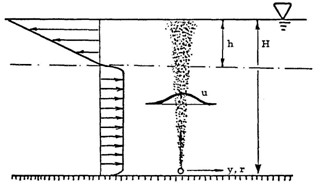Figure 1. Velocity field close to the air-bubble plume

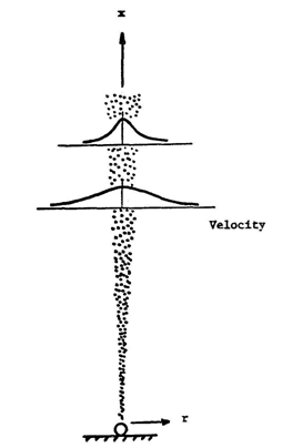Figure 2. Velocity field in air-bubble plume

Furthermore, the problem of predicting the moments of the distribution of bubble radius in bubbly flows is considered by (Tim et. al. 2008). The particular case where bubble oscillations occur due to a rapid (impulsive or step change) change in pressure is analyzed, and it is mathematically shown that in this case, inviscid bubble oscillations reach a stationary statistical equilibrium, whereby phase cancellations among bubbles with different sizes lead to time-invariant values of the statistics. It is also shown that at statistical equilibrium, moments of the bubble radius may be computed using the period-averaged bubble radius in place of the instantaneous one. For sufficiently broad distributions of bubble equilibrium (or initial) radius, it is demonstrated that bubble statistics reach equilibrium on a time scale that is fast compared to physical damping of bubble oscillations due to viscosity, heat transfer, and liquid compressibility. The period-averaged bubble radius may then be used to predict the slow changes in the moments caused by the damping. A benefit is that period averaging gives a much smoother integrand, and accurate statistics can be obtained by tracking as few as five bubbles from the broad distribution. The period-averaged formula may therefore prove useful in reducing computational effort in models of dilute bubbly flow wherein bubbles are forced by shock waves or other rapid pressure changes, for which, at present, the strong effects caused by a distribution in bubble size can only be accurately predicted by tracking thousands of bubbles. Some challenges associated with extending the results to more general (nonimpulsive) forcing and strong two-way coupled bubbly flows are briefly discussed (Tim et. al. 2008).

Moreover, the dispersion of gases through submerged orifices or nozzles plays an important role in enhancing the transport rates between phases in many chemical and physical processes. In many industrial heat exchange operations, a condensable gas is often injected into a liquid through a submerged orifice or nozzle to increase the rate of heat transfer between the gas and liquid, as direct contact heat transfer has the advantage of high heat transfer coefficient. (Denekamp et al. 1972, Cho and Lee 1990, and Chen and Tan 2001) have studied vapor bubble formation at submerged nozzle in its own liquid, that is, the processes studied involve only one component. When the dispersed and continuous phases are formed by two different immiscible components instead of one component, a two-phase particle can be observed during bubble formation. It contains a liquid and a vapor phase, the vapor accumulating in the inner part of the particle. Being neither a pure drop nor a pure vapor phase, this two-phase bubble has been referred to as a drobble (Sudhoff et al., 1982). The latter system differs from the former, one-component, system in that the condensate remains within the confines of the bubble envelope.

Owing to their wide application in industrial heat-transfer processes, two-phase bubbles have been extensively studied both experimentally and theoretically. (Sideman and Hirsch 1965) photographed condensing isopentane bubbles in water during their free rise period, or after their release from the nozzle. By analyzing consecutive pictures of each run, the instantaneous surface area, volume and vapor content of a rising drobble could be determined and the heat flux and transfer coefficients obtained. (Jacobs et al. 1978) proposed a model for the collapse of a bubble rising through a cold continuous immiscible liquid. (Wanchoo 1991) investigated the condensation of a rising two-phase bubble in immiscible liquid and derived an analytic expression for the steady rate of heat transfer from a two-phase bubble condensing in an immiscible liquid medium. (Wanchoo et al. 1997) measured experimentally the velocity of rise and the drag of a single vapor bubble collapsing in another immiscible liquid. (Sudhoff et al. 1982) reviewed the published studies since 1963 on the condensation or evaporation of a drobble and summarized the overall heat-transfer coefficients measured for various systems. More recently, (Kalman and Ullmann 1999) conducted a series of experiments of direct-contact condensation to the initial volume of a condensing bubble released from an orifice and the instantaneous shapes of drobble during the collapse process. Their experimental results showed that the initial volume of the condensing bubble could be reasonably predicted by employing Ruff’s two-stage model (Ruff 1972) that was originally developed for noncondensing bubbles.

Most of the above studies deal with the collapse of condensing drobble after its release from the nozzle. However, it is known that the period of bubble formation can contribute significantly to the overall heat and mass transfer of the process. (Terasaka et al. 1999) proposed a method to measure the heat-transfer coefficient for direct-contact condensation during two-phase bubble formation and theoretically estimated the direct-contact heat-transfer coefficient. (Terasaka et al. 2000) proposed a drobble for motion model to study the effect of operating conditions on two-phase bubble formation behavior at single nozzle submerged in water.

Two-phase bubble formation coupled with phase change at a submerged nozzle is studied theoretically. The whole bubble consists of a vapor and a liquid phase. The inner vapor phase is assumed to be surrounded by a thin condensate layer, in which the vapor condenses partially as the two-phase bubble grows. The interface element approach is applied to describe the dynamics of bubble formation. The effect of heat transfer from bulk vapor within the bubble to the surrounding bulk liquid is related to pressure analysis of vapor within the two-phase bubble via the mass flux of condensation. The results computed from this model agree well with the experimental data (Chen and Reginald 2003).

Beyond that, two-phase simulations may do an acceptable job of reproducing the near-field dynamics of bubble plumes, but they may also demand more resources than are feasible for computing the flow created by multiple plumes. In a practical setting, where computational fluid dynamics (CFD) might otherwise be used to investigate arrays of bubble diffusers for large-scale mixing applications, there arises the need for a plume model that can be easily incorporated into existing single-phase CFD codes. This need with a simple approximation for bubble-induced vertical acceleration inside an idealized cylindrical plume was accommodated, without solving additional equations of motion for the bubbles themselves (Robert et. al. 2000).

Earlier single-phase models (T. Deb Roy et. al. 1978, J. H. Grevet et. al. 1982, D. Mazumdar and R.I.L. Guthrie 1985, A. H. Castillejos et. al. 1989, D. Balaji and D. Mazumdar 1991) have employed fixed cylindrical or conical plumes, within which all the bubbles remain as they rise toward the surface. In such models, the buoyant acceleration of the surrounding liquid is proportional only to the volume of undissolved gas inside the idealized plume, and (Mazumdar and Guthrie 1994) have demonstrated that approximations of this sort can render velocity predictions outside the plume that are as accurate as those of two phase models. Although a conical plume is qualitatively more realistic, a cylindrical model was proposed by (Robert et. al. 2000) because it is easier to implement for multiple plumes, and simplicity is a practical consideration when the model is to be used in designing arrays of two or more bubble diffusers to mix large volumes of liquid. For applications of the latter kind, in which velocity prediction is much more important outside the plume than inside, the author demonstrated that a cylindrical column is an adequate representation for bubble plumes in unstratified liquids (Robert et. al. 2000).

On the other hand, local characteristics of flow and phase distribution are crucial to model and enhance mass transfer flux in multiphase reactors, but difficult to acquire.

Flows in bubble reactors may be complex and chaotic, all the more when these reactors are used under relevant industrial operating conditions. They usually show heterogeneous bubbling regime: the high gas flow rate generates bubble swarms and large intense liquid vortices, leading to high level of turbulence and highly distorted bubbles.

In these severe conditions, it is therefore difficult to perform reliable experimental investigations. Non-invasive techniques, like camera imaging or tomography techniques (Boyer et. al. 2002), cannot be applied, due to large pilot dimensions, high gas hold-up and highly fluctuating flow. Wall pressure transducers seem to be appropriate to most gas–liquid processes; however, they usually provide space averaged values only (mean gas hold-up between the axial positions of two transducers).

Use of invasive techniques is also critical: due to pressure or corrosive fluids, it may be difficult to settle probes through pilot wall. What is more, most of the invasive techniques require specific precautions that may not be consistent with reactor operating conditions. For instance, hot film anemometry can be used in two-phase flows for investigation of gas hold-up and liquid velocity (Utiger et. al. 1999 and Larue 2001), but a strict temperature uniformity is necessary to derive reliable velocities. Classical Pitot tubes have to be flow oriented (Bruun 1995), which is quite impossible to achieve in recirculating flows.

To get various local characteristics of gas phase, optical fibre probes are often chosen (Schweitzer et. al. 2001). These probes can be very thin but also quite robust if needed. This technique directly provides local gas hold-up and bubbling frequency even if the sensor is not strictly flow oriented. With a specific signal treatment and under some assumptions, it may also derive bubble velocity and bubble size (Werther 1974, Clark et. al. 1988 and Revankar and Ishii 1992). But the assumptions to be made are restrictive: exclusively vertical bubble motion, isotropy of turbulence and regular bubble shape (spherical or ellipsoidal). This kind of treatment has been tested for chains of distorted tumbling bubbles (Chaumat et al. 2005). In this case, bubble velocity distributions can be obtained, provided that some adjustable parameters, linked to the range of expected bubble velocities, are well defined. However, bubble size distribution turns out to be very difficult to obtain, due to distorted shapes and chaotic motion of bubbles: these conditions are far from the classical hypothesis used for data treatment. Nevertheless, the mean bubble velocity and the mean Sauter diameter have been found more meaningful, because their derivation requires data of gas hold-up, bubble frequency and most probable velocity (issued from inter-correlation of both signals) only.

Whereas, predicting the motion of bubbles in dispersed flows is a key problem in fluid mechanics that has a bearing on a wide range of applications from oceanicography to chemical engineering. The recent progress made in describing bubble motion in inhomogeneous flow was synthesized. A trident approach consisting of experimental, analytical, and numerical work has given a clearer description of the hydrodynamic forces experienced by isolated bubbles moving either in inviscid flows or in slightly viscous laminar flows. A significant research is devoted to a discussion of drag, added-mass force, and shear-induced lift experienced by spheroidal bubbles moving in inertially dominated, time-dependent, rotational, non-uniform flows. The important influence of surfactants and shape distortion on bubble motion in a quiescent liquid is highlighted. Examples of bubble motion in inhomogeneous flows combining several of the effects mentioned above are discussed (Hassan 2002, 2003, 2006, 2011, 2012, 2013, Hassan and Tamer 2006, Abdulmouti, et. al. 2000, Hassan et. al. 1997, 1998, 1999- No. 1, 1999- No. 2 and 2001, Hassan and Esam, 2013, among others).

The bubble drag and lift coefficients, C_D and C_L, are of great importance in the numerical prediction of bubbly flows based on multi-fluid models (Tomiyama and Shimada 2001) and bubble tracking methods (Tomiyama et. al. 1997, 1998, 2001, Tomiyama 1998 and Zun et. al. 1993). Though a number of studies on C_D and C_L have been carried out so far (Clift et. al. 1998 and Magnaudet and Eames 2000). The knowledge on them is still insufficient even for single bubbles in stagnant liquids and in simple shear flows for lack of relevant experimental data such as the terminal velocities of single bubbles in various stagnant liquids and the lateral migration of single bubbles in viscous linear shear flows. Several fundamental experiments on single bubbles have therefore been conducted, such as measurements of:

(1) shapes and motions of single bubbles in various infinite stagnant liquids (Tomiyama et. al. 2001 and Tomiyama 2002).

(2) shapes and motions of single bubbles in various conduits (Tomiyama et. al. 2001 and Tomiyama et. al. 2002).

(3) lateral migration of single bubbles in linear shear flows of various liquids (Tomiyama 2002 and Tomiyama et. al. 2002).

(4) lateral migration of single bubbles due to the presence of wall(Tomiyama et. al. 2001 and Tomiyama 2002).

Theoretical and numerical works to develop reliable closure relations have been also carried out along with the experimental works (Tomiyama et. al. 2001, Tomiyama 2002, Tomiyama et. al. 2002). (Tomiyama 2002) reviewed recent studies on single bubbles carried out in laboratory. The necessary and sufficient condition of dynamical similarity for a single bubble was deduced from the local instantaneous field equations to make clear the forces acting on a bubble and relevant dimensionless groups for modeling the terminal velocity and drag coefficient. Then a theoretical terminal velocity model for oblate and prolate spheroidal bubbles was deduced from the local instantaneous equations and jump conditions. The lack of uniqueness in terminal velocity caused by a certain kind of nonlinear bifurcation of terminal condition was discussed. Then the effects of fluid properties, bubble sizes and shear rates on the lift coefficients of single bubbles in viscous linear shear flows were discussed by (Tomiyama 2002).

A simple approximation is proposed for the buoyant force in a bubble plume. Assuming a uniform radius and slip velocity for the entire bubble column, an expression is derived for the vertical acceleration of liquid in the column, which is directly proportional to the injected gas flow-rate and inversely proportional to depth and velocity. This bubble-induced acceleration has been implemented with a k-ε turbulence model in a three-dimensional, single-phase CFD code, whose numerical predictions indicate that the velocity outside the plume is relatively insensitive to the column radius and the bubble slip velocity. Using a median observed value of 25 cm/s for the bubble slip velocity, and a column radius given by an empirical formula based on the work of (Cederwall and Ditmars 1970), the model renders predictions for velocity that compare favorably with experimental data taken outside single and double plumes in water. Predicted velocity increases in less-than-linear fashion with the gas flow-rate, and the flow-rate exponent approaches 1/2 in the lower limit, and 1/3 in the upper limit. In the range of flow-rates (200-22,000 cm³/s) for which the model is validated herein, the exponent is roughly 2/5 (Robert et. al. 2000).

Furthermore, the variety of applications of bubble plumes has triggered a host of experimental contributions, aimed at determining time-averaged velocities in tanks ranging from 1 m in diameter up to sinkholes of 50 m in depth (Milgram, 1983). Needless to say, the interpretation and comparison of results coming from such a variety of scales is complex. In fact, the shape of containers, different tank sizes and geometries and the complex nature of the problem make the interpretation of results somewhat cumbersome. This is complex even in non-stratified conditions. Tools to extrapolate bubble-plume behavior in small tanks to big tanks are largely needed.

In addition, a steady bubble plume model is developed to describe a weak air (or oxygen) bubble injection system used for the restoration of deep stratified lakes. Since the model is designed for two modes of operation, i.e., oxygenation and artificial mixing, gas exchange between water and bubbles has to be included. The integral model is based on the entrainment hypothesis and a variable buoyancy flux determined by the local plume properties and the ambient water column. Fluxes of eight properties are described by nonlinear differential equations which can be numerically integrated. In addition, five equations of state are used. The model leaves open two initial conditions, plume radius and plume velocity. Model calculations with real lake water profiles demonstrate the range of applicability for both modes of operation. The model agrees reasonably well with field data and with laboratory experiments conducted by various investigators.

It is known that bubble plumes are used to enhance the mixing and thus improving water quality in lakes and reservoirs. Two previous numerical studies show that the turbulence dissipates between 15 and 30% of the available power. In the experiments, the fraction is less than 1% because some of the energy of the plume is used to generate waves on the water surface and the profiles used to compute the volume-averaged dissipation were relatively far from the bubble plume. Measurements of the dissipation e would help to improve models of bubble plumes. These measurements could be used to evaluate and adjust the k – ε model, in which the dissipation is used to compute the eddy diffusivity, the turbulence time scale, and the sink of turbulent kinetic energy as done by (Hamilton and Schladow 1997).

Despite the uses for data on the dissipation, measurements of turbulence quantities in bubble plumes are rare. Some researchers have measured turbulent kinetic energy and Reynolds stress, and later on, to our knowledge, ensemble-averaged dissipation profiles were measured.

(Lohrmann et al. 1994 and 1995) proposed that due to the relatively high temporal resolution and small sampling volume of the ADV, it is possible to measure field and prototype scales of turbulence. Turbulent kinetic energy (TKE), dissipation rate of this energy (ε) and Kolmogorov length scale are the turbulent parameters computed and analyzed.

On the contrary, many authors stressed the importance of thermal diffusion effect on the bubble dynamics, and among the many mathematical analyses of the thermal diffusion effect, the model of Prosperity is notable. With the development of computational methods, the study of the thermal diffusion has progressed rapidly. Kameda and Matsumoto took into account the thermal diffusion effect in their bubbly shock flow simulation by solving the full set of partial differential equations i.e., compressible Navier-Stokes equations for spherical bubbles. This is computationally demanding but they obtained good agreement with experiments. Recently Preston et al. proposed a reduced order model of diffusive effect on the bubble dynamics and showed its validity by comparing the results with computations of the full partial differential equations. Their model is applicable to practical, complex bubbly flow computations.

Whereas, rising gas bubbles are routinely used to agitate liquids of diverse composition ranging from pure water to molten metal, but bubble plumes themselves present a class of fluid dynamics problems that are complex enough to defy precise solution by any currently available means. Nevertheless, from an approximate standpoint, considerable progress has been made, first with analytical models (H.E. Kobus 1968, K. Cederwall and J.D. Ditmars 1970, J. H. Milgram 1983, N. P. Mazumdar and N. Islam 1996 and I. Brevik and R. Killie 1996) that employ pre-defined (Gaussian) distributions for bubble concentration and liquid velocity, and more recently with numerical simulations (T. Deb Roy et. al. 1978, J. H. Grevet et. al. 1982, D. Mazumdar and R.I.L. Guthrie 1985, A. H. Castillejos et. al. 1989, D. Balaji and D. Mazumdar 1991, M. Millies and D. Mewes 1995, Y.Y. Sheng and G.A. Irons 1995, S.-M. Pan et. al. 1997, E. Delnoij et. al. 1997, H.-J. Park and W.-J. Yang 1997, M.P. Schwaz and W.J. Turner 1988, M.R. Davidson 1990, A. Sokolichin and G. Eigenberger 1994, S. Becker et. al. 1994, M.P. Schwaz 1996) that compute these quantities from prescribed governing equations. Single-phase simulations (T. Deb Roy et. al. 1978, J. H. Grevet et. al. 1982, D. Mazumdar and R.I.L. Guthrie 1985, A. H. Castillejos et. al. 1989, D. Balaji and D. Mazumdar 1991) (also called quasi single-phase simulations (D. Mazumdar and R.I.L. Guthrie 1995) confine the rising bubbles to a predetermined axisymmetric plume, inside which an upward buoyant force is imposed on the surrounding liquid, with the latter regarded as a single continuous fluid. Two-phase simulations (M. Millies and D. Mewes 1995, Y.Y. Sheng and G.A. Irons 1995, S.-M. Pan et. al. 1997, E. Delnoij et. al. 1997, H.-J. Park and W.-J. Yang 1997, M.P. Schwaz and W.J. Turner 1988, M.R. Davidson 1990, A. Sokolichin and G. Eigenberger 1994, S. Becker et. al. 1994, M.P. Schwaz 1996) impose no such plume constraint and fall into two general categories. Eulerian-Lagrangian simulations (M. Millies and D. Mewes 1995, Y.Y. Sheng and G.A. Irons 1995, S.-M. Pan et. al. 1997, E. Delnoij et. al. 1997, H.-J. Park and W.-J. Yang 1997) employ a Lagrangian viewpoint for the bubbles, tracking them as discrete particles, and an Eulerian viewpoint for the liquid, which is regarded as a continuous fluid. In contrast, Eulerian-Eulerian simulations (M.P. Schwaz and W.J. Turner 1988, M.R. Davidson 1990, A. Sokolichin and G. Eigenberger 1994, S. Becker et. al 1994, M.P. Schwaz 1996) use a volume-averaged approach in which the liquid and gas are treated as distinct, but continuous, fluids. Balaji and Mazumdar (D. Balaji and D. Mazumdar 1991) review single-phase models in particular, and (D. Mazumdar and Guthrie 1995) do likewise for single-phase and two-phase models in general. (Jakobsen et al. 1997) offer an extended review comparing the two different types of two phase models (Robert et. al. 2000).

Although efforts to compute the motion of multiphase flows are as old as CFD, the difficulty in solving the full Navier–Stokes equations in the presence of a deforming phase boundary has proven to be considerable. Progress was therefore slow and simulations of finite Reynolds number multiphase flows were limited to very simple problems for a long time. In the past few years, however, major progress has been achieved (Tryggvason 2001).

The oldest and still the most popular approach to comput multifluid and multiphase flows is to capture the front directly on a regular, stationary grid. The marker-and-cell (MAC) method, where marker particles are used to identify each fluid, and the VOF method, where a marker function is used, are the best known examples. Traditionally, the main difficulty in using these methods has been the maintenance of a sharp boundary between the different fluids and the computation of the surface tension. A number of recent developments, including a technique to include surface tension developed by (Brackbill et al. 1992), the use of subcells to improve the resolution of the interface (Chen et al. 1997), and the use of “level sets” (see, e.g., Sussman et al. 1994) to mark the fluid interface, have increased the accuracy and therefore the applicability of this approach. A review of the VOF method can be found in (Scardovelli and Zaleski 1999). The level-set method is reviewed by (Osher and Fedkiw 2001, Sethian 2001). Recent additions to the collection of methods that capture fluid interfaces on a fixed grid include the constrained interpolation profile (CIP) method of (Yabe 1997) and the phase-field method of (Jacqmin 1999). Both are reviewed in the issue (Jamet et. al. 2001 and Yabe et. al. 2001).

The second class of methods, and the one that offers potentially the highest accuracy, uses separate, boundary-fitted grids for each phase. The steady rise of buoyant, deformable, axisymmetric bubbles was simulated by (Ryskin and Leal 1984) using this method in a landmark paper that had a major impact on subsequent development. Several two-dimensional and axisymmetric computations of both the steady and the unsteady motion of one or two fluid particles or free surfaces can be found in the literature. This method is best suited to relatively simple geometries, and applications to complex fully three-dimensional problems with unsteady deforming phase boundaries are very rare. The simulation of a single unsteady three-dimensional bubble by (Takagi and Matsumoto 1994) is, perhaps, the most impressive example.

The third class is Lagrangian methods, where the grid follows the fluid. Examples of this approach include the two-dimensional computations of the breakup of a drop by (Oran and Boris 1987); the examination of the initial deformation of a buoyant bubble by (Shopov et al. 1990); simulations of the unsteady two-dimensional motion of several particles by (Feng et al. 1994 and 1995, and Hu 1996), and axisymmetric computations of the collision of a single drop with a wall by (Fukai et al. 1995). While this appears to be a fairly complex approach, (Johnson and Tezduyar 1997 and Hu et al. 2001)] have recently produced very impressive results for the three-dimensional unsteady motion of many spherical particles (Tryggvason 2001).

The fourth category is front tracking, where a separate front marks the interface but a fixed grid, only modified near the front to make a grid line follow the interface, is used for the fluid within each phase. The main developers of this approach are Glimm and collaborators (Glimm et al. 2001). In addition to front tracking methods that are, in principle, applicable to the full Navier–Stokes equations, specialized boundary integral methods have been used for both inviscid and Stokes flows. For a review of Stokes flow computations, (Pozrikidis 2001), and for a review of computations of inviscid flows, see (Hou et al. 2001).

The method presented by (Tryggvason et. al. 2001) is properly described as a hybrid between a front capturing and a front-tracking technique. A stationary regular grid is used for the fluid flow, but the interface is tracked by a separate grid of lower dimension. However, unlike front tracking methods, where each phase is treated separately, in (Tryggvason 2001) all the phases are treated together by solving a single set of governing equations for the whole flow field. Although the idea of using only one set of equations for many flowing phases is an old one, the method described by (Tryggvason 2001) is a direct descendant of a vortex-in-cell technique for inviscid multifluid flows described in (Tryggvason and Aref 1983 and Tryggvason 1988) and the immersed boundary method of (Peskin 1977) developed to put moving boundaries into finite Reynolds number homogeneous fluids. The original version of the method and a few sample computations were presented by (Unverdi and Tryggvason 1992).

This method has been used to examine many aspects of bubbly flows. (Unverdi and Tryggvason 1992) computed the interactions of two- and three-dimensional bubbles and (Jan 1994) examined the motion of two axisymmetric and two-dimensional bubbles in more detail. (Ervin and Tryggvason 1997 and Ervin 1993) computed the rise of a bubble in a vertical shear flow and showed that the lift force changes sign when the bubble deforms. The results of Jan and Ervin, which cover a rise Reynolds number range of about 1–100 have yielded considerable insight into the dependency of attractive and repulsive forces between two bubbles on the Reynolds number and bubble deformability. Preliminary studies of the interaction of bubbles with unsteady mixing layers are reported by (Taeibi–Rahni et al. 1994 and Loth et al. 1997). The motion of a few hundred two-dimensional bubbles at O(1) Reynolds number was simulated by (Esmaeeli and Tryggvason 1996), who found an inverse energy cascade similar to what is seen in two-dimensional turbulence. (Esmaeeli and Tryggvason 1998 and 1999) simulated the unsteady motion of several two- and three-dimensional bubbles, examining how the rise velocity and the bubble interactions depend on the Reynolds number.

More recently, (Bunner and Tryggvason 1999, 2000, 2002 and 2003) used a parallel version of the method to study the dynamics of up to 200 three-dimensional bubbles. Similar simulations of suspensions of drops have been done by (Mortazavi and Tryggvason 2000), who computed the motion of a periodic row of drops in a pressure-driven channel flow, and (Mortazavi 1995), who examined the collective behavior of many drops.

Another major effort has been the study of various aspects of sprays. The head-on collision of two axisymmetric drops computed by (Nobari et al. 1996 and Nobari and Tryggvason 1996) simulated the off-axis collisions of fully three-dimensional drops. Primary focus was on the case where the drops broke up again after initial coalescence. The numerical computations are in good agreement with available experimental data (for example, Jiang et al. 1992) and helped explain the boundary between the various collision modes. The binary collision of axisymmetric drops was examined again by (Qian et al. 1997), who focused on the draining of the film between the drops and compared the results with those of experiments. The capillary breakup of a liquid jet injected into another liquid was examined by (Homma et al. 2000 and Song and Tryggvason 1999) simulated the formation of a thick rim on the edge of a thin liquid sheet. An extensive study of the secondary breakup of drops has been done by (Han and Tryggvason 1999) and the primary atomization of jets, where the drop size is much smaller than the jet diameter, has been examined by (Tryggvason and Unverdi 1999, Tauber and Tryggvason 2000 and Tauber et al. 2002). Other related problems include simulations of the three-dimensional Rayleigh–Taylor instability by (Tryggvason and Unverdi 1990), an examination of the coalescence and mixing of two initially stationary drops by (Nobari 1993), and a study of the dissipation of surface waves by (Yang and Tryggvason 1998).

In addition to problems where two or more incompressible and immiscible fluids flow together, (Tryggvason et. al. 2001) have examined a number of problems where the governing physics is more complex. Simulations of the motion of bubbles and drops with variable surface tension, both due to temperature gradients and contamination are reviewd. Other simulations with complex surface forces include those of (Agresar et al. 1998), who modeled the response of a biological cell to various flows conditions, and (Che 1999), who computed the motion and deformation of drops resulting from electrostatic forces. The methodology has been extended in several studies to flows with phase change where the front moves relative to the fluid. (Juric and Tryggvason 1996) developed a method for the solidification of pure materials that accounts for the full Gibbs–Thompson conditions at the phase boundary and used it to examine the growth of dendrites. (Juric 1996) extended the method to simulate an unstable solidification front in binary alloys. A simpler solidification model, freezing the liquid as soon as the temperature drops below the melting temperature, allowed (Che 1999) to examine the solidification of multiple hot drops deposited on top of each other. In these computations, both phases had the same density. Generally, however, phase change is accompanied by local expansion at the phase boundary. The collapse of a cavitating bubble in a shear flow was examined by (Yu et al. 1995), who simply set the pressure inside the bubble equal to the vapor pressure of the liquid. A simple model of the combustion of a premixed flame, where the local expansion rate and thus the relative expansion velocity is a prescribed constant, was developed by (Qian et al. 1998) and used to examine the flame generation of vorticity. A more sophisticated method for the complete simulations of boiling was developed by (Juric and Tryggvason 1997).

Attempts to simulate multiphase flows go back to the early days of CFD at Los Alamos. While a few successful simulations can be found in the early literature, major progress has been made in the past few years. The “one-field” formulation is the key to much of this progress. The method described by (Tryggvason 2001) is one of the most successful implementations of the one-field formulation but impressive results have also been obtained by improved VOF methods, level-set methods, phase field methods, and the CIP method. The key difference between these methods and the technique described (Tryggvason 2001) is that (Tryggvason 2001) use of a separate “front” to mark the phase boundary, instead of a marker function. While explicit front tracking is generally more complex than the advection of a marker function, (Tryggvason et. al. 2001) believed that the increased accuracy and robustness are well worth the effort. The explicit tracking of the interface not only reduces errors associated with the advection of a marker function and surface tension computations, but the flexibility inherent in the explicit tracking approach should also be important for application to problems where complex interface physics must be accounted for (Tryggvason 2001).

The front-tracking method described by (Tryggvason 2001) is about 10 years old, although a number of refinements have been made as (Tryggvason et. al. 2001) have gained more experience in using it. During this time, other approaches have been developed and new ways have emerged to reduce and eliminate some of the limitations of methods like the one described by (Tryggvason et. al. 2001). (Cortez and Minon 2000), for example, have shown that it is possible to achieve higher accuracy and a faster convergent rate by the use of more sophisticated interactions between the front and the grid, and (Popinet and Zaleski 1999, Lock et al.1998, Udaykumar et al. 1999), and others have attempted to eliminate the smoothing of the front, while keeping most of the simplicity of the method described by (Tryggvason 2001). Although none of these authors have attempted three-dimensional calculations yet, the power of explicit tracking to facilitate increased accuracy is already clear. Recent progress in incorporating solid boundaries into methods based on fixed grids will also extend the utility of the method. For recent work on both stationary boundaries and boundaries with prescribed motion see (Fadlun et al. 2000). It is also likely that the approach used by (Glowinski et al. 2001) for freely moving solid objects in the fictitious domain method can be used in immersed boundary methods (Tryggvason 2001).

Direct numerical simulations of multiphase flows, using a front-tracking method, are presented by (Tryggvason 2001). The method is based on writing one set of governing equations for the whole computational domain and treating the different phases as one fluid with variable material properties. Interfacial terms are accounted for by adding the appropriate sources as δ functions at the boundary separating the phases. The unsteady Navier–Stokes equations are solved by a conventional finite volume method on a fixed, structured grid and the interface, or front, is tracked explicitly by connected marker points. Interfacial source terms such as surface tension are computed on the front and transferred to the fixed grid. Advection of fluid properties such as density is done by following the motion of the front. The method has been implemented for fully three-dimensional flows, as well as for two-dimensional and axisymmetric ones. First, the method is described for the flow of two or more isothermal phases. The representations of the moving interface and its dynamic restructuring, as well as the transfer of information between the moving front and the fixed grid, are discussed. Applications and extensions of the method to homogeneous bubbly flows, atomization, flows with variable surface tension, solidification, and boiling are then presented (Tryggvason 2001).

On the other hand, various experimental investigations have already been performed in bubbly flows, especially confined bubbly flows, in pipes, in 2D plumes and in bubble columns (Hassan et al., 1992; Rensen and Roig, 2001; Delnoj et al., 1999). Comparatively fewer studies were focused on non-confined or weakly confined bubbly flows (Milgram, 1983; Kobus, 1968). Various effects, including the presence of walls, may make the plume centerline, as well as the boundaries of the plume oscillate in three dimensions. Such effects may also change the two-phase flow behavior, producing strong coherent structures drifting in the dispersed phase. Moreover, the dissipation of large-scale motions resulting from buoyancy forces depends on the boundary conditions, so a careful control of the initial conditions is needed in performing such experiments.

The following conclusions can be drawn from the previous research in this area. For an air-water system, the spreading of the plume cross-sectional area was found to be approximately (but not exactly) linear (Tacke et al., 1985) depending on the 0.78 power of the elevation and proportional to the gas flow rate (Johansen et al., 1988). For nonaqueous experiments, instead, the spreading was not linear but increased with a power of 0.56 of the elevation (Tacke et al., 1985) and the plume spreading angle was about 9-10° smaller than that in air/water. Nevertheless, for a flow of argon in molten steel, the spreading cone angle was found to be 20° as in aqueous experiments (Szekely et al., 1979). For air/water conditions, the flow was observed to be highly three-dimensional (Milgram 1983; Castello-Branco and Schwerdtfeger, 1994; Koria and Singh, 1989), with plume precession and swirling occurring also at relatively low gas flow rates (Kuwagi and Ozoe, 1999; Johansen et al., 1988).

The radial distributions of bubble frequency and gas volume fraction were found to be essentially Gaussian (Tacke et al., 1985), while for the liquid velocity profiles, (Johansen et al., 1988) results were found to deviate from the Gaussian profile, perhaps because of the tank size employed in the particular experiments. (Anagbo and Brimacombe 1990) defined the profile as sigmoidal, increasing with the axial coordinate and decreasing with the radial one. Concerning the gas velocity, according to (Castillejos and Brimacombe 1987), three zones can be identified: in the region close to the injection, there is a steep radial gradient in bubble velocity, and the motion of the bubbles is strongly affected by the gas injection velocity and mode of injection; in the fully-developed flow region, the mean bubble velocity, and the standard deviation of the bubble velocity spectrum, exhibit relatively flat radial profiles, and the bubbles affect the flow only through buoyancy. Close to the liquid surface, the axial bubble velocity decreases more rapidly as liquid begins to flow radially outwards from the plume. The same changes in bubble behavior near the inlet were observed by (Anagbo and Brimacombe 1990), for injection through a porous plug. The slip velocity between the bubbles and the liquid is well represented by the terminal rising velocity of the same size bubbles in stagnant liquid, as has been found also by (Sheng and Irons 1995).

(Marco 2005) presented an extensive study of the most important hydrodynamic characteristics of fairly large-scale bubble plumes, created in a cylindrical vessel having a diameter of 2 m with water depth of 1.5-2 m. The bubbles were produced near the bottom of the vessel by a multi-needle circular injector having a diameter of 0.3 m. Several measurement techniques and a variety of tools were used to measure and to analyze the data. Particle Image Velocimetry (PIV), double-tip Optical Probes (OP), photographic techniques and three-dimensional Electro-Magnetic Probes (EMP) were extensively applied to measure bubble and liquid velocities, void-fraction, interfacial area concentration, bubble size and liquid re-circulation rates. PIV measurements in a vertical plane crossing the center of the injector provided the instantaneous velocity fields for both phases, including selected hydrodynamic parameters, such as the movement of the plume axis and its instantaneous cross-sectional width. Statistical studies were performed using image processing to determine the diameter and the instantaneous centerline position distributions and their fluctuations in time. An important finding was that there is not much instantaneous spreading of the plume. The stress tensor distributions obtained from the instantaneous data indicate that for the continuous phase, these stresses scale linearly with the local void-fraction in the range of 0.5 %< α <2.5%. The bubbles were found to be approximately ellipsoidal, with shape factor e ≈0.5 an equivalent bubble diameter (Sauter) of about 2-2.5 mm (Marco 2005).

The limitations imposed by measuring successively the flow parameters in each phase were eliminated. Indeed, since the velocities of the continuous and discrete phases are strongly correlated, simultaneous velocity measurements are required to estimate correctly the relative velocity. The PIV system was expanded with a second camera, used to measure simultaneously the velocity fields of the two phases in the vertical plane crossing the injector. In addition, a two-camera video recording system, stored simultaneous images of the 3D bubble plume structure so that the PIV data could be categorized according to the state of the plume (position and width). The instantaneous bubble and liquid velocity vector plots were correlated with the corresponding instantaneous bubble plume images. This allowed sampling and ensemble averaging of according to the bubble plume position or bubble plume diameter. The three dimensional plume dynamics was intensively investigated. The large-scale instability of the bubble plume resulted from meandering of the plume structure around its axis with superimposed horizontal cross-section fluctuation (Marco 2005).

The plume meandering and the horizontal cross-section fluctuation, supplied the instantaneous measured quantities with a coherent contribution which appeared as a fluctuation over the mean value. The coherent contribution to the globally time-averaged quantities such as velocities, Reynolds stress terms and therefore to the turbulence intensity was evaluated; the results showed a negligible contribution close to the injector and a substantial one at higher elevations. The coherent contribution was significant in both phase velocities, but stronger in the Reynolds stress terms and therefore in the turbulence properties (Marco 2005).

Moreover, a numerical scheme for bubble trajectories including their collisions is developed by (Arman et. al. 2007). An Eulerian-Lagrangian computational scheme is used to study the bubble trajectories. The 3D averaged Navier-Stock equations are solved. The SIMPLEC algorithm is used to relate the pressure to velocity. A one-way coupling is assumed and the effects of the bubbles on the carrier flow are neglected. The bubble equation of motion includes the drag, buoyancy, pressure gradient, Saffman lift and bubble volume change forces. The variation of the bubble radius is modeled using the Rayleigh-Plesset equation. The Kraichnan model is used to simulate the instantaneous turbulence fluctuation velocities. The hard sphere collision model is used to model the bubble collisions and the effects of bubble rotations are neglected. Trajectories of micro-bubbles in the near wall region are investigated, and the rate of collisions and the bubble deposition rate are studied. The results are compared with other simulations and good agreement is observed (Arman et. al. 2007).

On the other hand, bubbly flow can be found in many chemical and pharmaceutical industrial fluid flow applications such as in bubble columns and aerated stirred reactors. In order to accurately predict bubbly flows by using numerical methods, reliable interaction models as well as accurate representation of the continuous phase turbulence are required. (Dragana et. al. 2007) considered a bubble column. For the gas phase the Lagrangian Particle Tracking (LPT) method is used, and Large Eddy Simulation (LES) is applied for the liquid phase (Dragana et. al. 2007).

Using a combination of LES and LPT may in some applications lead to conflicting requirements on the resolution of the computational grid. In LES the resolution should be well within the inertial subrange of the energy spectrum. Often the Taylor micro-scale is used as recommended value. LPT, on the other hand, requires that effects of the bubbles should be considered as local, i.e. from a computational point of view the bubble is approximated as a point source. Hence, the bubble volume should be much smaller than that of a computational cell. However, in many industrial applications, for example stirred bioreactors, there is a fairy wide range of bubble sizes present and these are often in the same order of magnitude as the Taylor micro-scale. The requirements for LPT will then not be met leading to a less accurate solution (Dragana et. al. 2007).

(Dragana et. al. 2007) combined LES for the liquid phase and LPT for the gas phase to investigate the performance of LPT in the limit of large bubbles. Especially to investigate the proposed strategy in order to determine the potential for increasing the accuracy of the solution. This includes for example understanding the influence on the solution of different ways of distributing the effects of the dispersed phase on the finer grid levels. Hence, special handling of the gas phase is required if the bubbles are large (i.e. close to the grid resolution). The multi-grid structure of in-house CFD software of (Dragana et. al. 2007) was utilized in order to solve for the different phases on different grid resolutions, thereby meeting the requirements from both LES and LPT and thus improving the accuracy of the solution. Hence, the continuous phase flow is solved on the finest grid level available. The dispersed phase is solved on some coarser level where the resolution is in agreement with the LPT-requirements. The effects of the dispersed phase is then introduced as source terms in the momentum equation and transferred back to the finest grid using the multi-grid algorithm. The method is evaluated for bubble sizes in an intermediate range between the ranges where the LPT is valid and invalid. The large structures and the turbulent kinetic energy of the flow was studied and compared to experimental data (Deen 2001). Also, the effects on gas hold-up for varying superficial gas-velocity bubble diameter are considered. The test case is a square sectioned bubble column (W×W×H=0.15×0.15×0.45 m) with air bubbles injected into water through a sparger at the bottom of the column. The time averaged liquid velocity for different grid resolutions is compared to experimental data (Deen 2001). The L/h=28 resolution show a slight asymmetric velocity profile. The reason for that might be that sampling time is not sufficient to capture the low frequency oscillations of the plume (Dragana et. al. 2007).

On the contrary, due to their relative simplicity, their high contact efficiency and their good mixing properties, bubble column reactors are used in many chemical and petrochemical processes. In particular, the Fischer-Tropsch kind of reactions can be implemented in a bubble column reactor. To be economically viable, their implementation involves very large column diameters. Until now, experimental investigations have been carried out in cold flow columns with diameters up to 1 meter. With the purpose of designing of a new reactor, two important parameters are needed: the centre line velocity and the axial diffusion coefficient. Several correlations giving these design relevant parameters have been proposed by many authors. However, these correlations show large discrepancies at higher diameters that are industrially used. Because experimentation at larger diameters is very expensive, CFD simulations of bubble columns represent a useful alternative (Abdelhakim et. al. 2007).

A CFD commercial code (Fluent 6) has been used by (Abdelhakim et. al. 2007) to simulate the two-phase flow. A 2D non stationary Euler-Euler two-phase model is considered. Because the flow is buoyancy driven, the interaction between the liquid phase and the gas phase needs to be carefully modeled. Accordingly, a drag law that takes into account the effect of the bubble deformation and the gas volume fraction is implemented. A lift force has also been added and modeled using the model proposed by (Tomiyama and al. 2002).

However, the bubble diameter should be known in order to compute the interaction between the two phases. Therefore a population balance equation has been introduced to evaluate the Sauter mean diameter of the bubbles which is used in the interaction law. A model of (Luo and Svendsen 1996) which takes into account the coalescence and break-up of the bubbles is used in parallel with a discrete description of the population. The initial distribution is uniform. The initial bubble diameter is obtained using a correlation developed by Gaddis and (Vogelpohl 1993). Many simulations have been carried out by (Abdelhakim et. al. 2007) for a 1m column diameter and for different gas flow conditions. Simulation results are compared to their experimental data obtained with air and water. The CFD model compares favorably in terms of the global holdup and especially the velocity which approach satisfactorily the experimental values. The use of a discrete population balance model along with a relevant drag coefficient model allows the prediction of the velocity at the axis of the column with a good precision close to 10%. When adding a model for the lift force, the results are not better. The liquid centerline velocity which is an important parameter for the design of a bubble column reactor is overestimated (Abdelhakim et. al. 2007).

An accurate prediction of two-phase flow behavior in light water reactors during normal operation and accident conditions is essential to the reactor operation and safety, in particular for the advanced passive light water reactor designs. The two-fluid model is considered as the most detailed model due to its explicit treatment of the two phases. Past experiences, however, indicated that the accuracy of code predictions relies heavily on the constitutive relations in the two-fluid model, such as the interfacial area concentration, interfacial drag, etc. The interfacial area concentration is one of the geometric parameters that characterize the capability of the interfacial transfer of mass, momentum, and energy between the two phases, and needs to be accurately modeled (Xia and Xiaodong 2007).

In the past decade, a dynamic approach, namely, interfacial area transport equation (IATE), has been under development to take into account the bubble coalescence and disintegration, bubble nucleation, evaporation, and condensation (Kocamustafaogullari and Ishii, 1995; Millies et al., 1996; Wu et al., 1998; Yao and Morel, 2004). As a result, one-group and two-group IATEs have been developed, respectively, for bubbly flow and flow regimes beyond bubby flow, such as cap-bubbly, slug flow, and churn-turbulent flows (Ishii and Sun, 2006).

In (Xia and Xiaodong 2007) study, an attempt is being made to implement the one-group IATE into a CFD code, namely, FLUENT, in which the bubble size is not dynamically modeled. In the one-group IATE, the pressure effect on the gas expansion, bubble coalescence due to bubble random collisions driven by turbulence, bubble coalescence due to wake entrainment, and bubble disintegration caused by turbulent eddy impact have been modeled. Currently, the interfacial area concentration is introduced as a user defined scalar and the one-group IATE is implemented to solve for the scalar. The interfacial area concentration is then linked with the source terms of the two-fluid model conservation equations. Under this approach, the bubble size is dynamically modeled through its relation with the interfacial area concentration and void fraction.

Preliminary results indicate that FLUENT predicts the radial distribution of the void fraction in upward bubbly flow more accurately compared to that without the IATE. An air and water are introduced from the bottom into a vertical pipe of 50.8 mm inner diameter and a length of 3.1 m with superficial gas and liquid velocities of 0.13 and 0.49 m/s, respectively (Hibiki et al., 2001). The void fraction wall peak measured in the experiment is qualitatively captured by the current approach with the IATE while the original FLUENT code shows an opposite trend in the region close to the pipe wall.

A population balance model was developed in close cooperation of ANSYS-CFX and Forschungszentrum Dresden and implemented into CFX-10 (Frank et al. 2005, Krepper et al. 2007). (Eckhard et. al. 2007) presents the application of the model to bubbly upward flow in vertical pipes for air/water and for steam/water bubbly flow. The experiments were performed at FZ Dresden-Rossendorf. Radial gas volume fraction profiles, the bubble size distribution and the gas velocity are measured by wire mesh sensors (Eckhard te. al. 2007).

Gas-liquid flow in vertical pipes is a very good object for studying the corresponding phenomena. The bubbles move under clear boundary conditions, resulting in a shear field of nearly constant structure where the bubbles rise for a comparatively long time (Eckhard te. al. 2007).

The measured and calculated radial gas fraction distribution in an air/water bubbly flow in a DN200 pipe 7.802 m above the gas injection was presented. The superficial velocity for water, JW=1.067 m/s and for gas JG=0.14 m/s were specified. Two dispersed gaseous phases with a total of 21 size fractions were considered. The radial profiles of the gas fraction with respect to the two velocity groups were shown (Eckhard te. al. 2007).

In the vertical tube steam/water tests at saturation temperature i.e. with limited mass exchange between the phases were performed. Compared to air/water tests the critical bubble size of changing the lift force sign shifts towards smaller values. The model is able to calculate the correct distribution of the radial gas volume fraction. Applying the bubble break-up approaches suited for air/water flow also to steam/water flow, the bubble break-up is overestimated (Eckhard te. al. 2007).

The application to a bubbly flow around a half moon shaped obstacle arranged in a 200 mm pipe is shown by (Frank et al. 2007). The obstacle creates a pronounced three-dimensional two-phase flow field. The flow field was investigated in detail by varying the distance between the wire mesh sensor and the obstacle. CFD calculations applying the inhomogeneous MUSIG approach are presented in detail. The streamlines for the two dispersed phase groups was shown. The separation process of the bubbles also plays an important role here for the correct simulation (Eckhard te. al. 2007).

Applying the inhomogeneous MUSIG approach a more deep understanding of the flow structure is possible. While the closure models on bubble forces, which are responsible for the simulation of bubble migration, are in agreement with the experimental observations, clear deviations occur for bubble coalescence and fragmentation (Eckhard te. al. 2007).

(Monahan and Fox, 2007) showed that predictions of bubble-column flow regimes are highly dependent on the model formulation, which includes drag, added-mass (Cvm), lift (C), a bubble-pressure model (CBP), and a bubble-induced turbulence (BIT) model (CBT). The numerical simulations require the bubble-pressure term in order to predict homogeneous flow at high gas holdup as observed in the experiments of (Harteveld 2005). In (Sarah et. al. 2007) work, linear stability analysis (LSA) is performed for the full three-dimensional model to examine the dependence of flow instabilities on model parameters.

(Sarah et. al. 2007) showed that horizontal modes are strongly stabilized by certain combinations of C^BP and C, and identify two types of vertical instabilities: Type A, corresponding to the classical one-dimensional analysis of (Jackson 2000), and Type B, instability or turbulent profiles at large holdups due to a large positive lift relative to added-mass, bubble pressure, and turbulent dispersion. Type A modes can be stabilized by the parameter C_BP, though the minimum value required increases with increasing gas holdup. Type B instabilities result from the counteracting effects of bubble pressure and positive lift. Simulations show that the flow profiles exhibit distinctly different dynamics depending on which mode is unstable, and that large-scale instabilities seen experimentally are most likely associated with Type B instabilities. For Type B, the stabilizing function of the bubble-pressure model drives bubbles from regions of higher holdup to regions of lower holdup. However, the lift force drives bubbles from regions of lower holdup to regions of higher holdup, which destabilizes the flow. Increasing the effective viscosity dampens flow instabilities, but this would not happen if BIT were sufficiently suppressed. Thus, when the effect of positive lift is greater than that of the bubble pressure, the flow becomes unstable.

A possible scenario of (Sarah et. al. 2007) for transitions from homogeneous to heterogeneous flow at high holdups (as reported by Harteveld, 2005) is that bubble wakes are suppressed as gas holdup increases. Qualitatively, this would correspond to a decrease in BIT. Lowering CBT until the Type B modes become unstable (while keeping Type A modes stable) yields a transition from uniform to turbulent flow at high gas holdup ( α_d0~0.5) for positive lift (C~1). This scenario differs from that reported by (Lucas et al. 2006), who concluded that flow instabilities require negative lift. It also differs from the scenario reported by (Sankaranarayanan and Sundaresan 2002) for which columnar structures were observed in the cooperative-rise regime. In (Sarah et.a l. 2007) model, rise velocity is independent of gas holdup (as in the experiments of Harteveld, 2005).

A critical mode analysis shows that Type B instabilities originate in the horizontal components of the continuous- and dispersed-phase velocities. LSA predictions for the full 3D model were compared with simulations, and then use the simulations to explore the flow structure after a Type B instability (Sarah et. al. 2007).

In addition, detailed numerical simulations have been performed to study the effect of gravity on two-phase flow heat transfer (without phase change) in small diameter pipes by (G. Larrignon et. al. 2007). Effect of the flow orientation with respect to gravity is investigated. Overall, the heat removal rate in two-phase flow was shown to be significantly higher than in single phase flow. The downstream flow can be characterized as a periodic flow around each bubble/slug rather, where the shapes of the inclusions and the flow around them reach a repeatable state. The flow regime, viz. bubbly, slug, and slug-train is found to have a strong influence on the heat transfer and pressure drop. The wall thermal layer is affected by the blockage effect of the inclusions, which manifests itself in a circulating liquid flow pattern superimposed on the equivalent single-phase fully developed flow. The Nusselt number distribution shows that the bubbly, slug, and slug-train regimes transport as much as three to four times more heat from the tube wall to the bulk flow than pure water flow. For the flow against gravity, the breakup into bubbles/slugs occurs earlier and at a larger frequency, although the average Nusselt number is not significantly different. A mechanistic heat transfer model is proposed, based on frequency and length scale of inclusions (G. Larrignon et. al. 2007).

Moreover, the bubble size distribution (BSD) in a square bubble column is experimentally determined by the use of interferometric particle imaging (IPI) by (Rolf et. al. 2007). The method is a relatively new imaging technique for determining the diameter of spherical transparent particles from out-of-focus images, and the strength of the IPI technique is its ability to measure the instantaneous bubble diameter and velocity of spatially distributed bubbles (Madsen 2006).

The experiment is done on a square cross-sectioned bubble column with the dimensions 0.15 m × 0.15 m × 1 m (D × W × L). The column is built in Plexiglas, so that optical access is possible. An investigation of the gas and liquid flow pattern in the bubble column has already been done by (Deen 2001) using PIV. The experimental equipment is a Dantec IPI/PTV setup at Aalborg University Esbjerg, which consists of a 120 mJ pulsed ND: YAG laser, two 8 bit CCD cameras, Flowmapper processor and relevant Dantec software (Flowmanager). The cameras and laser head are mounted on a 3D traversing unit, so it is possible to access the entire column (Rolf et. al. 2007).

When focusing a camera on a transparent bubble that has been illuminated by a coherent laser sheet, the scattered light will produce two bright spots or glare points on a Charged Coupled Device (CCD) chip. By defocusing the camera with respect to the bubble the two glare points will interfere to produce measurable fringes on a CCD array.

Spacing the diameter of the bubble can be found (Rolf et. al. 2007).

The results show a number mean diameter of 4.4 mm and a Sauter mean diameter of 6.0 mm in the reported field of view, which corresponds well with what is observed in the column. BSDs have been determined in different locations in the bubble column, and the mean diameters are hardly distinguishable. It is observed that the BSDs show two distinct peaks, which is due to noise problems. This could be one of the problems that have to be solved in order to be able to distinguish between the mean diameters and BSDs in the column (Rolf et. al. 2007).

On the contrary, atomic force microscopy (AFM) have been a very powerful tool to study the phenomena in nanoscale, but very few studies have been reported on bubble dynamics due to the undeveloped measurement techniques and the difficulty of manipulation of bubble production. Long-lived stationery nanobubbles (apparent diameters of about 20nm) were imaged by AFM using tapping mode after the bubbles were formed on a substrate that was first contact with ethanol and was subsequently exposed to water (Lou et. al. 2000). (Tyrrell and Attard 2002) acquired both bubble images (with 30nm width and 20 nm height) and force-distance curves of nanobubbles on hydrophobic glass over a range of pH conditions. (Zhang et. al. 2006) studied the effect of solutes on the stability and morphology of nanobubbles (with 300 nm width and 20-30nm height), such like mono- or multivalent salts, cation- or anionic and solution pH (Joe et. al. 2007).

(Joe et. al. 2007) developed a novel method using force – distance curves (f-d curves) and records the histories of bubble nucleation process on prepared surface with grown CNTs coated with 10 nm platinum so that the bubble dynamics through theoretical model can be obtained (Joe et. al. 2007).

The typical f-d curve between AFM tip and prepared surface in DI water and no bubble is formed was shown, and the f-d curve as the bubbles are formed using the catalytic reaction of 0.1% hydrogen peroxide solution (H2O2) to oxygen was presented. These force curves reveal the change of repulsive force and the distance of repulsive force boundary due to the existence of the bubble and thus the bubble size and physical properties such as elastic coefficient, surface tensions and etc can be obtained by theoretical analysis from reasonable model (Joe et. al. 2007).

The time series of f-d curves during the catalytic reaction and thus the bubble nucleation process was addressed. The repulsive force is ranged ~1-3 pN acted at the tip-sample separation of 0.4-1.5μm on the approach force curve, which indicates that the bubble is smaller than 1.5μm. The bubble nucleation period of ~5.6 secs was represented. The detailed analysis results were reported (Joe et. al. 2007).

3. Design of Bubble Columns

The principle goal in bubble column design is to produce bubbles of an appropriate size, and the desirable hydrodynamic flow conditions. A system that is mass transfer limited (i.e. the rate of chemical reaction is high), for example, requires a large amount of interfacial area, and hence the generation of smaller bubbles with a correspondingly higher voidage. These conditions lead to decreased circulation in the column, however, which reduces the liquid phase heat and mass transfer coefficients (Harteveld 2005). The design of bubble column reactors is plagued by conicts such as (Deckwer 1985).

The contemporary design of bubble columns commonly involves the use of multiphase CFD codes. Several approaches have been developed for the numerical modeling of bubbly flow; these may be broadly grouped into three categories (Bove 2005):

(i) Eulerian/Eulerian models. Both phases are treated as continuum (i.e. no spatial separation of the phases is enforced). A population balance model may be coupled with the two-fluid model for tracking the evolution of the bubble size (Wang and Wang 2007).

(ii) Eulerian/Lagrangian models. This approach solves the continuous phase as a continuum, however bubbles are individually tracked. This approach is computationally limited to systems of no more than 10⁶ bubbles at present (Bove 2005).

(iii) Interface tracking models, such as the volume of fluid approach (Krishna and van 1998). This technique provides an accurate description of the interface between two fluids, however becomes too computationally intensive for systems of more than 100 bubbles (Bove 2005).

(Borchers et al. 1999) focused on flows with a central gas inlet. They varied the aspect ratio of the columns. They observed a mainly stationary state for aspect ratios smaller than 1.5. In that case, one major circulation cell fills the entire diameter of the column. For larger aspect ratios, a periodically meandering bubble plume was observed. Large vortices are moving down in the liquid next to the bubble plume. The period of the bubble plume movement turned out to be about 34 s. (Chen et al. 1989) made streak photos of the flow in a flat bubble column at a gas superficial velocity of 35 mm s-1. For different aspect ratios, they observed a pattern of staggered vortices which corresponds well with the observations of (Borchers et al. 1999).

(Becker et al. 1999) performed measurements in a system comparable to that of (Borchers et al. 1999). The main difference is that the column has other dimensions. The aspect ratio, L/D is larger than 1.5 and they observed a meandering bubble plume, which is in correspondence with the observations of (Borchers et al. 1999). They observed an oscillation period of about 17 s. They noted that the use of another sparger can reduce the oscillation period by 2 s.

Experiments of the flow of a bubble plume in a 3-D bubble column were performed by (Deen et al. 2000). Their experiments comprise a central plume rising in a column with an aspect ratio of 3. A meandering plume was observed. However, in contrary to the plumes in the flat bubble columns, which moved in a quasi-periodic fashion, the bubble plume in the 3- D column seems to be moving randomly. It was also observed that the presence of bubbles introduces large turbulent fluctuations in the liquid phase. The measured slip velocity between the gas and the liquid phase was in the order of 0.2 m s^-1.

3.1. Inuence of Dopants on Bubbly Flow

In a pure solution, the gas-liquid interface cannot support any stress and is completely mobile. This permits interphase momentum transfer, which generates recirculating vortices within rising bubbles: decreasing drag and increasing the bubble terminal velocity.

Further, liquid films between approaching bubbles are able to rapidly drain, which allows bubble coalescence to readily occur. These behaviors are dramatically altered in aqueous systems, however, by the presence of surface active molecules (Takagi and Matsumoto 2011). Surfactants (i.e. organic molecules composed of a hydrophobic non-polar segment, typically an aliphatic chain, and a hydrophilic polar functional group, such as a hydroxyl) tend to adsorb at the interface, where the hydrophobic tail extends into the gas phase, while the hydrophilic head resides in the water. These surfactants lower the surface tension, which decreases bubble sizes and thus increases liquid hold-up. By accumulating at the interface the surfactant molecules alter the interfacial shear condition, which can range from the formation of a `rigid cap', as the surfactants are swept to the rear of the bubble as it rises, to a no-slip boundary condition covering the entire surface of bubble for heavily contaminated systems (Takagi and Matsumoto 2011). This loss of interfacial mobility leads to increased skin friction, which slows the bubble rise velocity. Further, the adsorbed surfactants introduce Marangoni forces that slow the film drainage process, and hence hinder bubble coalescence and stabilize bubbly flow at higher voidages (Ruzicka et. al. 2008).

While the inuence of organic surfactants on gas-liquid flows is well known, the impact of inorganic molecules is less well understood. It is well established that the presence of inorganic ions at moderate concentrations can either increase or decrease the surface tension of water (Weissenborn and Pugh 1996), which can have a stabilizing inuence on bubbles. At concentrations lower than that required to significantly alter the surface tension, however, some (but not all [Craig 2004 and Henry et. al. 2007]) inorganic salts still exert a strong inuence on the behaviour of bubbly flow.

It has been observed by many authors that a small concentration of salt greatly decreases bubble coalescence (Marrucci and Nicodemo 1967, Lessard and Zieminski 1971, Zieminski and Whittemore 1971, Kelkar et. al. 1983, Jamialahmadi and Muller 1992, Deschenes et. al. 1998, Ruthiya et. al. 2006, Ribeiro and Mewes 2007 and Orvalho et. al. 2009), with this phenomenon attributed to a slowing of the film drainage process (Marrucci 1969 and Zahradnk 1997). These effects are noted to only occur above a certain transitional concentration, at which point a step-change in the stability of bubbly flow occurs (Ribeiro and Mewes 2007 and Zahradnk et. al. 1997). While it is known that the inuence of electrolytes is ion specific (Craig 2004 and Henry et.al. 2007), it remains contested in the literature whether low concentrations of electrolyte have an inuence on the dynamics of single bubbles, with (Henry et al. 2009 and Sato et al. 2010) claiming no effect, while (Jamialahmadi and Muller 1992) stating that salt slows bubble rise. The mechanisms of bubble stabilization by inorganic dopants are not well understood; (Zieminski and Whittemore 1971) discuss the possibility of ion-water interactions, which render the film between bubbles more cohesive, while, (Craig et al. 1993) discuss suggest some form of hydrophobic interaction.

3.2. Measurement of Bubble Size and Interfacial Area

The measurement of bubble size distributions is highly desirable, as it is the property which governs the bubble rise velocity and hence the residence time in a given unit operation. The measurement of interfacial area is also important, as it is the property which (when multiplied by some driving force) governs rates of interphase mass, momentum and energy transfer.

Many techniques have been developed for the measurement of bubble size. Most prominent are photographic techniques, which are reviewed by (Tayali and Bates 1990). This approach involves obtaining photographs of bubbly flow through a transparent section of the column. Several improvements to the basic technique have been suggested, such as shadowgraphy, which removes the inuence of the position of bubbles within the column by projecting bubble shapes onto an opaque medium, such that the focal length of the camera is the same for all bubbles. Bubble sizes were measured in this way by (van den Hengel 2004 and Majumder et al. 2006). Due to the occlusion of the dispersed phase in the bulk flow, however, these optical techniques are typically limited to relatively low gas-fractions. Also commonly used are acoustic techniques, wherein the frequency of pressure variations in the column (caused by either passive or driven bubble shape oscillations) are measured and used to infer bubble size. The acoustic measurement of bubble size is reviewed in full by (Leighton 1997). Like optical techniques, however, acoustic measurements fail at higher voidages, where the pressure uctuations in the column are increasingly dominated by bubble-bubble interactions (Manasseh et. al. 2001). For low voidage systems, the acoustic technique was found to be more accurate than optical measurements (by comparison with volumetric measurements on bubbles captured in a funnel) (Vazquez et. al. 2005). This reacts the problem of obtaining a true measurement of bubble volume from 2D projections of a bubble, as discussed by (Lunde and Perkins 1998).

To permit bubble size measurements in high voidage systems, many invasive probes have been developed. These typically consist of single or multi-point electrical conductivity or fibre optic local phase probes, as reviewed by (Saxena et al. 1988). These probes have been employed in many studies (Magaud et. al. 2001, Hibiki et. al. 2003 and Kalkach et. al. 1993). The systematic error generated by the intrusive nature of these problems has been the subject of much work; a comprehensive review of which is provided by (Julia et al. 2005). More recently, wire-mesh sensors have become popular for their two dimensional visualization capability (Prasser et. al. 2001 and 2007). While these sensors possess excellent time resolution (on the order of thousands of frames per second), they are currently limited to a spatial resolution on the order of 1 mm, which is insufficient for the accurate determination of bubble size distributions. Additionally, the errors associated with the distortion of bubble shape due to the wire mesh are to be explored in full, and in this case, as the mesh is completely destructive to the structure of the two phase flow, wire mesh sensors cannot be used for measurements which explore the evolution of the dispersed phase.

Several tomographic techniques have been explored for the characterization of gas-liquid flows, however finding a workable balance between temporal and spatial resolution has proved difficult. Electrical tomographies (including electrical resistance tomography, electrical capacitance tomography and electrical impedance tomography) have been investigated, however, despite having extremely short acquisition times, are of far too low spatial resolution for the identification of individual bubbles (Wang et. al. 2010). A range of radiographic tomographies, reviewed by (Chaouki et al. 1997), has also been explored. In particular, computer aided x-ray tomography has been widely tested; however the need to mechanically rotate the emission source around the sample decreases the time resolution below that required. To overcome this problem, ultra-fast x-ray scanners, which use a number of fixed emission sources, have been developed, however the limited number of emitters and detectors employed to date has reduced the spatial resolution below that required for the accurate measurement of bubble size (Prasser et. al. 2005). Most recently, (Bieberle et al. 2009) have demonstrated the use of an auspicious alternative method of x-ray tomography. In their technique, Bieberle et al. scan an electron beam back and forth across a block of tungsten, which emits x-rays through a bubble column to a ring of detectors on its opposite side. This permits temporal resolutions on the order of milliseconds to be achieved, while imaging at a spatial resolution of approximately 1 mm. Thus this technique demonstrates spatial and temporal resolutions on the same order of magnitude as wire mesh sensors, with the additional advantage of being non-invasive. With further refinement to yield higher resolution images, this technique may be very useful for the measurement of bubble size and shape in high voidage systems, particularly if the high temporal resolution of the technique can be exploited for the rapid production of 3D images (Alexander 2011).

The measurement of interfacial area is closely related to that of bubble size, with an estimate of surface area able to be calculated from measured bubble sizes by assuming some bubble shape. To improve the accuracy of the measurement of interfacial area, therefore, it is desirable to also measure some information about bubble shape. Beyond optical techniques at low void fractions, the measurement of bubble shape is very difficult. Some work has focused upon the determination of bubble shape from chord lengths which may be measured using local phase probes (Kulkarni et. al. 2004). Alternatively, spatially averaged interfacial area may be determined for a system undergoing chemisorption by measuring the concentration of the reactants at various points in the column. Common chemisorption systems used for this purpose are discussed by (Deckwer 1985).

3.3. Measurement of Liquid-Phase Hydrodynamics

Bubbly flow is a hydrodynamically complex system. The entrainment of fluid with the rising bubbles leads to the formation of large scale recirculation vortices (Mudde 2005), which govern liquid-side mass and heat transfer. Much work has focused on the quantification of liquid phase velocities in bubbly flow, with a broad range of experimental techniques being developed. Hot film anemometry, wherein the local fluid velocity is determined around a heating element by measurement of the heat flux (Bruun 1996), was the first technique to be explored. Like local phase probes, however, hot film anemometry is highly intrusive; the errors associated with the invasive nature of the probe are discussed by (Rensen et al. 2005). As an alternative, laser Doppler anemometry (LDA) has found considerable use (Becker et. al. 1994, 1999 and Borchers et. al. 1999). This technique measures the light scattered by small seed particles as they flow through an interference pattern generated by two intersecting laser beams or laser sheets. LDA may also be used to infer a measurement of bubble size (Kulkarni et. al. 2004). PIV, which uses high-speed cameras to track the motion of seed particles, has also recently increased in popularity, and has been applied to the study of bubble flow (Delnoij et. al. 2000). Both LDA and PIV are, however, optically based, which limits the applicability of the techniques to low voidage systems. The highest gas-fraction bubbly flow system to which optical velocimetry has been applied was of voidage 25%, however those authors reported an exponential decrease in sampling rate as they sampled further from the column wall (Mudde et. al. 1997). To overcome the optical limitation, a variant of PIV has been proposed that uses x-rays and x-ray absorbing seed particles (Seeger et. al. 2001), while phase contrast x-ray velocimetry techniques have also been demonstrated (Kim and Lee 2006). Lastly, a computer aided radioactive particle tracking technique (CARPT) has been applied to bubbly flow by (Devanathan et al. 1990). In this technique, a single radioactive particle is allowed to circulate in a bubble column, and by tracking the particle's position over several hours the time averaged flow field inside of the column can be determined.

Magnetic Resonance Imaging (MRI) is therefore a very a promising technique for application to bubbly flow systems, as it avoids these two problems entirely. Further, MRI can be used to produce both structural images and quantitative velocity maps of a system (Fukushima 1999). There exist fairly limited applications of magnetic resonance to bubbly flow in the literature, and most studies produce only temporally or spatially averaged measurements. Bubbly flows were first examined using magnetic resonance by (Lynch and Segel 1977), who used spatially averaged measurements to quantify the void fraction present in their system. They demonstrated a linear dependence between NMR signal and volume-averaged gas fraction. (Abouelwafa and Kendall 1979) subsequently used a similar technique to estimate the voidage and flow rate of each phase. (Leblond et al. 1998) used pulsed field gradient (PFG) NMR (a technique for the measurement of molecular displacement) to quantify liquid velocity distributions for gas-liquid flows and obtained some measurement of the flow instability. (Barberon and Leblond 2001) applied the same technique to the quantification of flow around singular Taylor bubbles and were able to demonstrate the existence of recirculation vortices in the bubble's wake. (Le Gall et al. 2001) also used PFG NMR to study liquid velocity uctuations associated with bubbly flow in different geometries. (Daidzic et al. 2005) obtained 1D projections of bubbly flow with a time resolution of approximately 10 ms, however, due to hardware limitations, were only able to produce time averaged 2D images. Similarly, temporally averaged 2D measurements were acquired by (Reyes 1998), who examined gas-liquid slug flow, and by (Sankey et al. 2009), who investigated bubbly flow in a horizontal pipe. Most recently, (Stevenson et al. 2010) used gas-phase PFG NMR to size bubbles in a butane foam, and (Holland et al. 2011) produced a Bayesian technique for determining bubble sizes from MRI signals. The only study in the literature which demonstrates MRI measurements with both temporal and spatial resolution on a gas-liquid system is that of (Gladden et al. 2006), who presented velocity fields in the vicinity of a Taylor bubble.

(Alexander 2011) describes the first application of ultra-fast magnetic resonance imaging (MRI) towards the characterization of bubbly flow systems. The principle goal of his study is to provide a hydrodynamic characterization of a model bubble column using drift-flux analysis by supplying experimental closure for those parameters which are considered difficult to measure by conventional means. The system studied consisted of a 31 mm diameter semi-batch bubble column, with 16.68 mM dysprosium chloride solution as the continuous phase. This dopant served the dual purpose of stabilizing the system at higher voidages, and enabling the use of ultra-fast MRI by rendering the magnetic susceptibilities of the two phases equivalent (Alexander 2011).

Spiral imaging was selected as the optimal MRI scan protocol for application to bubbly flow on the basis of its high temporal resolution, and robustness to fluid flow and shear. A velocimetric variant of this technique was developed, and demonstrated in application to unsteady, single-phase pipe flow up to a Reynolds number of 12,000. By employing a compressed sensing reconstruction, images were acquired at a rate of 188 fps. Images were then acquired of bubbly flow for the entire range of voidages for which bubbly flow was possible (up to 40.8%). Measurements of bubble size distribution and interfacial area were extracted from these data. Single component velocity fields were also acquired for the entire range of voidages examined (Alexander 2011).

The terminal velocity of single bubbles in the system was explored in detail with the goal of validating a bubble rise model for use in drift-flux analysis. In order to provide closure to the most sophisticated bubble rise models, a new experimental methodology for quantifying the 3D shape of rising single bubbles was described. When closed using shape information produced using this technique, the theory predicted bubble terminal velocities within 9% error for all bubble sizes examined. Drift-flux analysis was then used to provide a hydrodynamic model for the present system. Good predictions were produced for the voidage at all examined superficial gas velocities (within 5% error), however the transition of the system to slug flow was dramatically over predicted. This is due to the stabilizing inuence of the paramagnetic dopant, and reacts that while drift-flux analysis is suitable for predicting liquid holdup in electrolyte stabilized systems, it does not provide an accurate representation of hydrodynamic stability (Alexander 2011).

Finally, velocity encoded spiral imaging was applied to study the dynamics of single bubble wakes. Both freely rising bubbles and bubbles held static in a contraction were examined. Unstable transverse plane vortices were evident in the wake of the static bubble, which were seen to be coupled with both the path deviations and wake shedding of the bubble. These measurements demonstrate the great usefulness for spiral imaging in the study of transient multiphase flow phenomena (Alexander 2011).

3.4. MRI Theory

In late 1945, a group of researchers at Harvard University, led by (Purcell et. al. 1946), almost simultaneously with (Bloch et. al. 1946 and contemporaries working independently at Stanford University, showed that certain nuclei could absorb and subsequently emit radiofrequency (r.f.) energy when placed in a magnetic field at a certain nuclei-specific strength. These were the first observations of the phenomenon known as nuclear magnetic resonance (NMR). Purcell and Bloch were awarded the Nobel Prize for their discovery in 1952, which has since developed into a routine technique for chemical analysis. In 1973, Lauterbur and Mansfield and Grannell showed that by application of a spatially variable magnetic field, the position of the emitting nuclei could be determined. This was the foundation of magnetic resonance imaging (MRI). (Mansfield 1977) subsequently developed MRI for applications in medicine, and MRI has since become one of the most potent medical diagnostic tools available today. Most recently, MRI has emerged as a useful tool for research in the natural sciences and engineering, where it is enabling measurements unavailable to previous generations of researchers (Alexander 2011).

4. Two-Fluid Euler-Euler Model

Experimentally it is difficult to obtain detailed information about the interactions of the bubbles with each other and the flow. Such information can, however, be obtained by direct numerical simulations (DNS), where the governing equations are solved numerically on sufficiently fine grids so that every continuum length and time scales are fully resolved. Such studies of single-phase flows have a long history, whereas DNS of multiphase flows, where it is necessary to account for the moving phase boundary, are more recent. DNS of homogeneous buoyant bubbles can be found in the works done by (Esmaeeli and Tryggvason 1998, 1999 and 2005, Bunner and Tryggvason 2002 and 2003) for example. Recently, (Lu, Biswas, and Tryggvason 2006) numerically examined laminar bubbly flows in a vertical channel. The results showed that for nearly spherical bubbles, the lateral migration of the bubbles due to lift resulted in two regions: A core where the void fraction is such that the weight of the liquid/bubble mixture balances the imposed pressure gradient (and the velocity is therefore constant) and a wall layer that is free of bubbles for downflow and bubble-rich for upflow. The velocity profile can be computed analytically for laminar downflow, but for upflow the exact profile (and therefore the total velocity increase) depends strongly on the deformability of the bubbles. The flow in the core, including the rise velocity of the bubbles, is well described by results for homogeneous flows.

The derivation of the model equations for the two-phase bubbly flow starts with the assumption that both phases can be described as continua, governed by the partial differential equations of continuum mechanics. The phases are separated by an interface, which is assumed to be a surface. At the interface, jump conditions for the conservation of mass and momentum can be formulated (Ishii, 1975, Drew 1983). The direct solution of these microscopic equations supplemented by appropriate initial conditions would yield a complete description of the two-phase flow. This approach is called direct numerical simulation (DNS). Since systems of practical interest usually comprise a large number of interacting bubbles, such problems are far too complicated to permit a direct solution. The application of DNS to the simulation of turbulent two-phase flow is thus restricted to the flow around a few gas bubbles (Lin et al., 1996; Tryggvason et al., 1998) and cannot be used for modeling of industrial-scale reactors.

In all cases where a flow is caused by the injection of gas bubbles into a liquid, the main flow driving force results from local density differences of the gas-liquid mixture that is differences in the local gas holdup. Like any buoyancy driven flow, such a flow situation is highly unstationary and characterized by a spectrum of fluctuating vortices of different size. Its mathematical representation, therefore, requires taking the full 3-D, dynamic model equations into account. The numerical solution of these detailed model equations, however, requires such a computational effort that up to now the detailed simulation and model-based design of gas-liquid reactors with bubbly flow like bubble columns or bubble column loop reactors has been severely impeded. It is, therefore, of prime importance to reduce the computational effort by reasonable simplifications of the hydrodynamics model. In this contribution, the two-fluid continuum approach was discussed by (A. Sokolichin et. al. 2004) where each volume element contains a mixture of gas and liquid, the mean density of which varies from element to element. Like in other buoyancy driven flows, the Boussinesq approximation for the momentum balance of the gas/liquid mixture proves to be reasonable. The mixture density changes are then neglected in all momentum terms and only considered in the buoyancy term. In addition, any displacement of liquid by gas was neglected in the liquid continuity equation. The resulting model for the hydrodynamics of the gas/liquid mixture is similar to a single-phase flow model and can be solved efficiently with the respective well established iterative solution procedure. The validity of these simplifications has been proved for several examples by comparison with detailed simulation results (A. Sokolichin et. al. 2004).

In the above solution procedure, the change of the local gas holdup has to be described by the solution of the gas-phase continuity and momentum equations. The latter requires the specification of the interaction forces between gas and liquid. Starting from the rise velocity of single bubbles, the pressure force and the drag force have been identified as most important. The added mass force proved to be negligible since the steady-state rising velocity for normal size bubbles in water is established within milliseconds. For buoyancy driven bubbly flow, lift forces have so far been used primarily to adjust steady state, 2-D simulation results to experiments. Since 3-D, dynamic simulations did not require an adjustment through additional lift forces, it is concluded that they are not essential for the simulation of the buoyancy driven bubbly flow. Since they are able to change the flow structure substantially, they should be omitted, as long as no clear experimental evidence of their direction and magnitude is available (A. Sokolichin et. al. 2004).

5. Significance to Fossil Energy Program

Converting coal to liquid hydrocarbon fuel by direct and indirect liquefaction processes has been of great concern to the development of coal-based energy systems. While the direct hydrogenation has been quite successful and was further developed in various forms, use of slurry phase Fischer-Tropsch (F-T) processing is considered a potentially more economical scheme to convert synthesis gas into liquid fuels. Slurry transport and processing and pneumatic transport of particles play a critical role in the operation, efficiency, safety and maintenance of these advanced coal liquefaction and coal-based liquid fuel production systems. Therefore, a fundamental understanding of reacting coal slurries will have a significant impact on the future of environmentally acceptable liquid fuel generation from coal (Goodarz 2004).

Particle-particle and particle-gas/liquid interactions strongly affect the performance of three-phase slurry reactors used in coal conversion processes and are crucial to the further development of coal-based synthetic hydrocarbon fuel production systems. The scientific knowledge base for these processes, however, is in its infancy. Therefore, most current techniques were developed on an ad hoc and trial and error basis. The needed fundamental understanding of the dynamics of chemically active slurries and three-phase mixtures is provided. In particular, a computational model for predicting the behavior of dense mixtures in coal liquefaction and liquid fuel production equipment were developed (Goodarz 2004).

Three-phase flows with liquids, bubbles, and solid particles occur in a wide range of industrial processes (Fan, 1989). Important applications include three-phase slurry reactors in coal conversion processes, and in particular, in synthetic liquid fuel production. Optimization of three-phase slurry reactors requires a fundamental understanding of multiphase hydrodynamics coupled with heat and mass transfer processes. Despite a number of investigations on multiphase flows, the three-phase slurry reactor technology is far from being matured with many critical unresolved issues (Goodarz 2004).

There are two main approaches to modeling multiphase flows that account for the interactions between the phases. These are the Eulerian-Eulerian and the Eulerian-Lagrangian approaches. The former is based on the concept of interpenetrating continua, for which all the phases are treated as continuous media with properties analogous to those of a fluid. The Eulerian-Lagrangian approach adopts a continuum description for the liquid phase and tracks the discrete phases using Lagrangian particle trajectory analysis (Goodarz 2004).

In recent years, a number of simulation results using Eulerian-Eulerian model were reported in the literature. For gas-particle flows, (Sinclair and Jackson 1989) studied gas-particle flows in a vertical pipe including particle-particle interactions. (Ahmadi and Ma 1990) developed a thermodynamical formulation for dispersed multiphase fluid-solid turbulent flows, which was used to study dense simple shear flows (Ma and Ahmadi, 1990). (Ding and Gidaspow 1990) developed a bubbling fluidization model using kinetic theory of granular flows. (Pita and Sundaresan 1993) performed numerical study on developing flow of a gas-particle mixture in a vertical riser. (Abu-Zaid and Ahmadi 1992) proposed a stress transport model for rapid granular flows in a rotating frame of reference. (Abu-Zaid and Ahmadi 1996) also developed a rate-dependent model for turbulent flows of dilute and dense two-phase mixtures. (Cao and Ahmadi 1995, 2000) reported their numerical simulation results for gas-particle two-phase turbulent flows in vertical, horizontal and inclined ducts. They accounted for the phasic fluctuation energy transport and interactions (Goodarz 2004).

For gas-liquid flows, (Gasche et al. 1990) developed a two-fluid model for bubble column reactors. (Torvik and Svendsen 1990, Svendsen et al. 1992, and Hillmer et al. 1994) included the effects of turbulence kinetic energy and the dissipation rate caused by the interaction between the two phases in their models. (Hjertager and Morud 1993, 1995) treated the liquid and gas phases as space-sharing interdispersed continua and described the interactions through interfacial friction terms. (Sokolichin et al. 1993, 1994) reported their simulations using Eulerian-Eulerian method. (Krishna et al. 1999) studied the influence of scale on the hydrodynamics of bubble columns using Eulerian-Eulerian model approach and a k-ε turbulence model. (Sanyal et al. 1999) studied gas liquid flows in a cylindrical bubble column using Eulerian-Eulerian approach and compared their result with algebraic slip mixture model. (Borchers et al. 1999) discussed the applicability of the standard k-ε turbulence model in an Eulerian-Eulerian approach for simulation of bubble columns. (Mudde and Simonin 1999) reported their two- and three-dimensional simulation of a meandering bubble plume using Eulerian-Eulerian method that included the k-ε turbulence model. Additional progress in simulating bubble columns were reported by (Rande 1992, Grienberger and Hofman 1992, Boisson and Malin 1996, Pfleger et al. 1999, Goodarz 2004).

The accuracy of Eulerian-Eulerian approach heavily relies on the empirical constitutive equations used. Furthermore, the approach has limitations in predicting certain discrete flow characteristics. For example, particle size effect, particle agglomeration or bubble coalescence and breakage cannot be fully accounted for. The Eulerian-Lagrangian model, however, involves smaller number of empirical equations and is more suitable for providing detailed information of discrete phases. The disadvantage of this approach is its requirement for more extensive computing time (Goodarz 2004).

The Eulerian-Lagrangian model has been widely used in two-phase flows. (Li and Ahmadi 1992, and Kvasnak and Ahmadi 1996) simulated the instantaneous turbulent velocity field across channels and ducts using an anisotropic Gaussian random field model. (Sommerfeld and Zivkovic 1992) reported a simulation of pneumatic conveying through pipe systems, in which they incorporated their particle-wall and particle-particle collision models. Using a model described by (Crowe 1977, Fan et al. 1997) performed numerical simulations of gas-particle two-phase turbulent flows in a vertical pipe. (Tsuji et al. 1993) provided a discrete particle simulation of two-dimensional fluidized bed using a soft particle model. Their model was further modified by (Hoomans et al. 1996 and Xu and Yu 1997) who developed hard sphere collision models. (Andrews and O’Rourke 1996, Snider et al. 1998) reported a multiphase particle-in-cell method for dense particulate flows. (Zhang 1998) conducted a simulation of gas-particle flows in curved ducts using particle-wall and particle-particle random impact models. (Patankar and Joseph 2001a, b) performed simulations of particulate flows using a Chorin-type fractional-step method for gas phase equations. (Fan et al. 2001) reported simulations of particle dispersion in a three-dimensional temporal mixing layer. They found that the particle dispersion patterns were governed by the large scale vortex structures (Goodarz 2004).

Early works based on Eulerian-Lagrangian simulation models for bubbly flows include those of (Webb et al. 1992, Trapp and Mortensen 1993, Lapin and Lubbert 1994, and Devanathan et al. 1995). (Sokolichin et al. 1996) compared the simulation results of Eulerian-Eulerian model and Eulerian-Lagrangian model with the experimental data, but neglected bubble-bubble interactions.

(Delnoij et al. 1997a,b) developed an Eulerian-Lagrangian model for a bubble column operating in the homogeneous flow regime. Their simulations incorporated bubble-bubble interactions using a collision model, but ignored bubble coalescence. (Lain et al. 1999) developed an Eulerian-Lagrangian approach including turbulence using the k-ε turbulence model. Their model, however, neglected the effect of phase volume fractions. More recently, ignoring bubble-bubble interactions, (Lapin et al. 2002) reported their Eulerian-Lagrangian simulations of slender bubble columns. Their prediction suggests that the flow moves downwards near the axis and rises close to the wall in the lower part of the column, but in the upper part the opposite trend is observed (Goodarz 2004).

While there is an extensive literature of two-phase flow model, studies of three phase flow hydrodynamics are rather limited. (Gidaspow et al. 1994) described a model for three-phase-slurry hydrodynamics. (Grevskott et al. 1996) developed a two-fluid model for three-phase bubble columns in cylindrical coordinates. They used a k-ε turbulence model and included bubble-generated turbulence. (Mitra-Majumdar et al. 1997) proposed a CFD model for examining the structure of three-phase flows through a vertical column. They suggested new correlations for the drag between the liquid and the bubbles and accounted for the particle effects on bubble motions. Recently (Wu and Gidaspow 2000) reported their simulation results for gas-liquid slurry bubble column using the kinetic theory of granular flows for particle collisions. (Padial et al. 2000) performed simulations of three-phase flows in a three-dimensional draft-tube bubble column using a finite-volume technique. (Gamwo et al. 2003) reported a CFD model for chemically active three-phase slurry reactor for methanol synthesis. However, all these models were based on Eulerian-Eulerian approach. Computer simulations of gas-liquid-solid flows using an Eulerian-Lagrangian model are rather limited. Recently, (Zhang 1999) performed a series of simulations of three-phase flow using VOF method for the liquid and the gas phases and a Lagrangian method for particles. Their study, however, were limited to consideration of only a small number of bubbles (Goodarz 2004).

An Eulerian-Largrangian formulation for analyzing three-phase slurry flows in a bubble column was developed by (Goodarz 2004). The approach used an Eulerian analysis of liquid flows in the bubble column, and made use of the Lagrangian trajectory analysis for the bubbles and particle motions. The bubble-bubble and particle-particle collisions are included the model. The model predictions are compared with the experimental data and good agreement was found. An experimental setup for studying two-dimensional bubble columns was developed. The multiphase flow conditions in the bubble column were measured using optical image processing and PIV. A simple shear flow device for bubble motion in a constant shear flow field was also developed. The flow conditions in simple shear flow device were studied using PIV method. Concentration and velocity of particles of different sizes near a wall in a duct flow was also measured. The technique of Phase-Doppler anemometry was used. An Eulerian VOF computational model for the flow condition in the two-dimensional bubble column was also developed. The liquid and bubble motions were analyzed and the results were compared with observed flow patterns in the experimental setup. Solid-fluid mixture flows in ducts and passages at different angle of orientations were also analyzed. The model predictions were compared with the experimental data and good agreement was found. Gravity chute flows of solid-liquid mixtures were also studied. The simulation results were compared with the experimental data and discussed A thermodynamically consistent model for multiphase slurry flows with and without chemical reaction in a state of turbulent motion was developed. The balance laws were obtained and the constitutive laws established (Goodarz 2004).

6. Laser Doppler Anemometry (LDA) in Dispersed Gas-Liquid Flow

Laser Doppler anemometry (LDA) is a widespread and much appreciated non-intrusive technique for measuring fluid dynamics in single-phase (gas or liquid) flow, e.g. in process technology or in aerodynamics, (Drain 1980; Adrian 1983; Durst et al. 1987; Absil 1995), in particular in studying highly turbulent flows, where the fluctuation intensity can be so high that other techniques such as hot wire anemometry face serious difficulties.

The applicability of LDA to two-phase flow, in particular to disperse gas-liquid (bubbly) flow, is the subject of ongoing debate. Though several studies have been presented on what can be measured in certain special well-deflned conditions (Groen et. al. 1999), what is needed is insight into the applicability of LDA for measuring two-phase fluid dynamics in “real” two-phase flows in practical situations, such as in bubble columns (Groen et. al. 1999).

The fundamental issue that has to be addressed when applying LDA to dispersed two-phase flow is what exactly is being measured, i.e. the velocity of one of the phases (and if so, which one), or of both phases (and if so, to which extent which one). A further important question is whether or how this is being influenced by the experimental conditions or by the LDA configuration. An important issue herein is the question of what happens when the dispersed phase passes the measuring volume. In the case of gas-solid or liquid-solid dispersed flow, a solid particle generally has a surface rough enough to scatter light in any direction and hence to produce a valid burst onto the detector. However, in gas-liquid flow, because of the relatively reflecting rather than scattering nature of the bubble interface, the light is only sometimes directed towards the detector, therefore not always a velocity realization will be accomplished.

(Ohba et al. 1976a, b and Mahalingam et al. 1976) investigated the use of LDA in two-phase (gas-solid and gas-liquid) flow. (Durst ZareH 1975) studied the interference patterns of a laser beam scattered by surfaces (particles and bubbles) which are large with respect to the laser beam diameter. This was applied in relating the light scattering characteristics of single bubbles of up to 1 mm in diameter to their velocities (Martin et al. 1981; Martin and Chandler, 1982). This resulted in the so-called triple-peak technique, with which under well defined conditions it is possible to measure the velocities and sizes of passing bubbles (Brankovic et al. 1984, 1986; Yu and Varty 1988). The triple-peak technique holds for spherical bubbles in the range of 0.1-3.0 mm diameter (Currie and Brankovic 1987).

Often, LDA is used to explicitly measure the fluid mechanics of the liquid phase in two-phase flows, e.g. in dispersed gas-liquid flows (MarieH 1983 and of Lance and coworkers Lance and Bataille 1991; Lance et al. 1991), or of liquid entrained in a gas jet (Loth and Faeth 1989). (Durst et al. 1986) used a combined (forward and sidescatter) technique to study the flow around bubbles, bubble rise velocities and the effects of passing bubbles on the surrounding liquid.

Considerations for applying LDA to bubbly flows with bubbles about 3 to 4 mm in diameter were investigated by means of detailed experiments in the model geometry of a train of bubbles. Both forward scatter and backscatter LDA were studied. The validity of phase discrimination via burst amplitude was tested and special attention was paid to the impact of bubble interface response to the laser beams. Forward and backscatter measurements can be compared well. In both conflgurations, predominantly the liquid phase is “seen” by LDA. A bubble itself only leads to a velocity realization in special conditions. In those cases, the Doppler shift is determined by the motion of the bubble interface which consists of the motion of the center of gravity of the bubble as well as shape oscillations. In backscatter bubbles only give velocity realizations when their “cheeks” pass through the measuring volume virtually perpendicularly. It is shown that the bubble-caused velocity realization frequency is very low for bubbles of the size used. Phase discrimination on burst amplitude does not hold. In ambient cases such as bubble columns one can assume that only the liquid phase is being studied (Groen et. al. 1999).

Bubble induced gas-liquid flow is the basis of fluid movement in many chemical engineering devices and applications ranging from boilers or evaporators over two- or three-phase bubble column reactors of various design to large-scale aerobic (and sometimes anaerobic) sewage treatment plants. About 20 years ago, modeling and simulation of these systems was restricted to strongly simplified (overall) fluid- flow models, primarily because the computer power for the solution of more detailed models was not sufficient. In the meantime, a number of efficient commercial CFD-codes are available and the power of desktop PC or workstations is strong enough for quite detailed simulation studies (Sanyal et al., 1999; Krishna et al., 2000; Pfleger and Becker, 2001). In most cases reasonable to good agreement of experimental results and simulations has been shown or claimed, implying that the predictive power of CFD simulations for bubble flow is already a reliable level.

The last comprehensive reviews on the modeling of bubble driven flows were (Jakobsen et al. 1997, Joshi 2001, Joshi et al. 2002). They listed the different approaches for the modeling of bubble-liquid interaction forces and only briefly addressed bubble induced turbulence.

7. Application of Two Phase Boiling in Micro Channel

It is worth noting that what happens in microchannels is two-phase flow, which is quite different from single-phase flows in microchannels. Furthermore, many of the controlling phenomena and mechanisms change when passing from macrochannel two-phase flow and heat transfer to microchannels act. For example, surface tension (capillary) forces become much stronger as the channel size diminishes while gravitational forces are weakened. Therefore, it is usually not sensible to empirically refit macro scale methods to micro scale data since the underlying physics have substantially changed. This means that new dimensionless groups have come into play while the influence of others has disappeared (Sandhya 2007).

In recent years, the research in the field of single- and two-phase flow heat transfer at a micro scale level has been constantly increasing due to the rapid growth of the technology applications that require the transfer of high heat rates in a relatively small space and volume. (Suo and Griffith 1964) did the first study in micro Chanel of 1.03 and 1.60 mm diameter and observed three distinctive flow patterns: bubbly/slug, slug and annular flow. Their study covered heptane and water as the liquid phase, and helium and nitrogen as the gas phase. (Cornwell and Kew 1992) also noted three different flow patterns in rectangular channels (1.2 × 0.9 mm and 3.5 × 1.1 mm) for tests with R-113 and R-141b: isolated bubbles, confined bubbles, and slug/annular flow. He also postulated the concept of confinement number to note macro-to-micro transition.

Some authors as a further example, (Coleman and Garimella 1999) classified their observations into a total of 16 regimes subdivided into four main traditional groups (dispersed, intermittent, wavy and annular) that were then subdivided as follows: dispersed flow into 3 types of bubbly flow, intermittent flow into 4 types of slug and plug flow, wavy flow into 4 types of waves, and annular into 5 categories of annular films. Some very good photographs of the flow regimes are shown in their papers. (Yang and Shieh 2001) study on flow patterns of air-water and two-phase R-134a in small circular and was not able to predict different flow regimes for refrigerant flow. (Hetsroni et al. 2003) performed experiments for air-water and steam-water flow in parallel triangular microchannels and emphasized the discrepancy between flow patterns of air-water and steam-water flow.

An overview of the state-of-the-art of two-phase macro-to-micro scale transition criteria like bond number, confinement number and bubble departure diameter, two-phase flow patterns, void fractions and two-phase pressure drops in microchannels is described by (Sandhya 2007).

He addresses both experimental study for predicting two phase flow pattern regimes methods for micro channel and numerical expression to predict the frictional pressure drop across the micro channel. His objective of the investigation is to systematically study the gas liquid two-phase flow patterns, and pressure drop in capillaries with circular cross-sections (Sandhya 2007).

Numerous applications for micro scale flow boiling are emerging: high heat flux cooling of computer microprocessor chips and power electronics, precise cooling of micro-reactors, rapid and uniform cooling of LED displays, development of automotive evaporators with multi-port aluminum tubes, etc. All of these applications require thermal design methods that are accurate, reliable and robust (that is, methods that follow the trends of the data well and work for a multitude of fluids, channel sizes and shapes, pressures, flow rates, heat fluxes, etc.). Presently, the state-of-the-art is only partially able to fulfill such requirements in micro-channel heat sinks, channels are fabricated into the silicon chip (CPU), and coolant is pumped through them. The channels are designed with very large surface area which results in large heat transfers, further increased if two-phase flow cooling is applied (Sandhya 2007).

Rapid development of microfluidic devices has triggered the demand for a comprehensive understanding of the flow characteristics in microchannels to advance their design and process control. Micro scale devices can be fabricated using micromachining technologies and used for cooling microelectronic circuits, bioengineering applications, aerospace and micro heat pipes, among others. Some of these applications involve gas liquid two-phase flows in channels much less than 1 mm in diameter. The two-phase flow characteristics that need to be well understood include the two-phase flow regimes, void fraction and pressure drop.

From a point of view of applications, micro heat exchangers, micro cooling assemblies and thermal systems implementing such devices, referred to as micro-thermal-mechanical systems (MTMS) as opposed to micro-electronic-mechanical-systems (MEMS), are rapidly advancing to ever smaller sizes. These are used as micro cooling elements for electronic components, portable computer chips, radar and aerospace avionics components, and micro chemical reactors. Besides single-phase cooling applications, numerous two-phase (evaporation) cooling applications are being identified, for now being implemented without the benefit of thermal design methods for heat transfer and pressure drops (a difficult which is overcome by extensive testing). In fact, what can now be fabricated, either by micromachining of silicon wafers or micro extrusion of aluminum elements, has vastly outpaced what can be thermally modeled. In addition, while circular channels are the norm for macro scale evaporation processes, at the micro scale non-circular channels are more common. Thus, significant advances are required for the optimal development and operation of these devices (Sandhya 2007).

8. The Turbulent Bubbly Flow

Bubbly flows, which are observed in many industrial situations, are usually seen in a kind of turbulent condition. The turbulent behavior of the bubble flows is classified by many kinds of characteristic parameters, i.e., the scale of the flow field, the void distribution, large vortices, turbulent eddies, bubble volumes, and the wake length of the bubble. Moreover, as a basic study of the global behavior of a turbulent bubble flow and the micro scale flow structure of a bubble plume, which drives liquid convection due to its buoyancy, it was found that the bubble plume has a spiral structure depending on the bubble size and the void fraction. Also, the turbulent fluctuation is enhanced inside the plume due to the two-way interaction between the bubble motion and the surrounding liquid flow. (Hassan 2002, 2003, 2006, 2011, 2012, 2013, Hassan and Tamer 2006, Abdulmouti, et. al. 2000, Hassan et. al. 1997, 1998, 1999- No. 1, 1999- No. 2 and 2001, Hassan and Esam 2013, Murai and Matsumoto 1996).

In addition, the turbulent modulation in two-phase flows has drawn interest by many researchers over many years both from scientific and practical points of view. Although the size and the concentration of particles or bubbles are considered main factors of the turbulence modulation, attention has been paid mainly to the effect of the particles or bubble size on the turbulence modulation (Hassan 2002, 2003, 2006, 2011, 2012, 2013, Hassan and Tamer 2006, Abdulmouti, et. al. 2000, Hassan et. al. 1997, 1998, 1999- No. 1, 1999- No. 2 and 2001, Hassan and Esam, 2013, Gore and Crowe 1989, Serizawa et. al. 1975a, b, c, Theofanous and Sallivar 1982, Tsuji et. al. 1982, Tsuji et. al. 1984, Marie and Lance 1983).

Moreover, the turbulence induced by the bubble motion significantly governs the performance of agitation, chemical reactions and heat transfer. Hence, turbulence is one of the key parameters in understanding the thermal and hydrodynamic behavior of a gas-liquid flow. Particularly, in recent years, much more detailed analysis has become necessary in order to improve the performance and safety of industrial equipment’s utilizing gas-liquid two-phase flows. In this relation, information of two-phase flow turbulence becomes more and more important. Therefore, research on the turbulence in gas-liquid two-phase flow has been carried out for the recent decades both experimentally and theoretically. In the experiments on two-phase flow turbulence, one interesting phenomenon has been observed particularly in the bubbly flow regime. An analysis was made of the turbulence suppression phenomenon in the bubble two-phase flow, which is characterized by a smaller turbulent energy than that in single-phase flow. The turbulence generation term and the turbulence absorption term due to the bubble-eddy interaction are found to play the most important role in the turbulence suppression phenomenon of a bubbly flow (Hassan 2002, 2003, 2006, 2011, 2012, 2013, Hassan and Tamer 2006, Abdulmouti, et. al. 2000, Hassan et. al. 1997, 1998, 1999- No. 1, 1999- No. 2 and 2001, Hassan and Esam, 2013, Lance and Bataille 1991, Isao Kataoka et. al. 1993).

Furthermore, turbulent boundary layer skin friction in liquid flows may be reduced when bubbles are present near the surface on which the boundary layer forms. Prior experimental studies of this phenomenon reached downstream-distance-based Reynolds numbers (Rex) of several million, but potential applications may occur at Rex orders of magnitude higher.

(WENDY et. al. 2006) presented results for Rex as high as 210 million from skin-friction drag-reduction experiments conducted in the USA Navy's William B. Morgan Large Cavitation Channel (LCC). Where, a near-zero-pressure-gradient flat-plate turbulent boundary layer was generated on a 12.9 m long hydraulically smooth flat plate that spanned the 3 m wide test section. The test surface faced downward and air was injected at volumetric rates as high as 0.38 m3 s⁻¹ through one of two flush-mounted 40 μm sintered-metal strips that nearly spanned the test model at upstream and downstream locations. Spatially and temporally averaged shear stress and bubble-image-based measurements are reported here for nominal test speeds of 6, 12 and 18 m s⁻¹. The mean bubble diameter was ∼300 μm. At the lowest test speed and highest air injection rate, buoyancy pushed the air bubbles to the plate surface where they coalesced to form a nearly continuous gas film that persisted to the end of the plate with near-100% skin-friction drag reduction. At the higher two flow speeds, the bubbles generally remained distinct and skin-friction drag reduction was observed when the bubbly mixture was closer to the plate surface than 300 wall units of the boundary-layer flow without air injection, even when the bubble diameter was more than 100 of these wall units. Skin-friction drag reduction was lost when the near-wall shear induced the bubbles to migrate from the plate surface. This bubble-migration phenomenon limited the persistence of bubble-induced skin-friction drag reduction to the first few meters downstream of the air injector in the current experiments.

Moreover, the lubrication of external liquid flow with a bubbly mixture or gas layer has been the goal of engineers for many years. (Steven et. al. 2010) presented the underlying principles and recent advances of this technology. They reviewed the use of partial and super cavities for drag reduction of axisymmetric objects moving within a liquid. Partial cavity flows can also be used to reduce the friction drag on the nominally two-dimensional portions of a horizontal surface; they also presented the basic flow features of two-dimensional cavities. Injection of gas can lead to the creation of a bubbly mixture near the flow surface that can significantly modify the flow within the turbulent boundary layer, and there have been significant advances in the understanding of the underlying physical process of drag reduction. Moreover, with sufficient gas flux, the bubbles flowing beneath a solid surface can coalesce to form a thin drag-reducing air layer. (Steven et. al. 2010) discussed the current applications of these techniques to underwater vehicles and surface ship.

It is well known that when a small air bubble bursts from an equilibrium position at an air/ water interface, a complex motion ensues resulting in the production of a high-speed liquid jet. When a bubble bursts at a free surface, the surface tension rapidly pulls the rim where they intersect outward and downward. Eventually, a ring of fluid at the base of what was the bubble contracts to a point, throwing a plume of fluid upward in the form of a high-speed jet. The jet will often break up into a number of drops. The corresponding downward jet may be expected to advect vorticity from the separated boundary layer into the region beneath the bubble. Various aspects of this motion have been studied experimentally by a number of researchers. The free surface motion following the burst was modeled numerically using a boundary integral method (Garner Ellis and Lacey 1954). This has important implications for the boilogical industry where animal cells in bioreactors have been found to be killed by the presence of small bubbles. With respect to bubbles approaching a free surface, experimental and theoretical aspects are considered in a number of papers (Allan, Charles and Mason 1961). The effect of the approach speed of a bubble towards a free surface was investigated by (Kirkpatrick and Lochett 1974). (Kientzler et. al. 1954) showed pictures of the breakup of the high-speed liquid jet that follows a bubble burst. (Newitt Dombrowaski and Knelman 1954) showed that there are two types of drops released after the burst: large ones emanating from the jet and smaller ones from the liquid film above the bubble. This thin lamella breaks up into a number of tiny droplets, which are projected sideways by the expansion of the bursting film and upwards by the rush of gas as the pressure in the bubble is released. In a more comprehensive study, (MacIntyre 1972) showed that the film, as it breaks, 'rolls-up' into an expanding toroidal rim. This rim may break irregularly into a number of tiny droplets. He mentioned that this rim of the film is expanding too rapidly to be broken up by capillary ripples, as in the case of the jet. Instead, this breakup is due to the turbulence from the escaping air coupled with the effects of variations of surface tension and film thickness. What remains after bubble burst, of the toroidal rim follows a ripple down the sides of the bubbles, and it was shown that the liquid in the jet originates in a thin layer surrounding the bubble crater (Boulton-Stone and Blake 1993).

Beyond that, in turbulent boundary layer, kinetic energy from the free stream flow is covered into turbulent fluctuations and then dissipated into internal energy by viscous action. This process is continual, such that the turbulent boundary layer is self-sustaining in the absence of strong stabilizing effects. For as long as these facts have been known, fluid dynamics have sought to understand just how boundary-layer turbulence is generated at the expense of the mean motion, and just how it is dissipated. These are the objectives of studying the internal structures of turbulence. Since boundary-layer flows are the technical driver for so many engineering applications, immense human and financial resources have been brought to bear on the problem over many decades of study (Robinson 1991).

The air bubble plume induced by the steady release of air into water has been analyzed with an integral technique based on the equations for conservation of mass, momentum and buoyancy. This approach has been widely used to study the behavior of submged turbulent jets and plumes. The case of air-bubble induced flow, however, includes additional features. The compressibility of the air and the differential velocity between the rising air bubbles, and the water are introduced as basic properties of the air - bubble plume in addition to a fundamental coefficient of entrainment and a turbulent Schmidt number characterizing the lateral spreading of the air bubbles.

The liquid turbulence structure of air-water bubbly flow in a 200 mm diameter vertical pipe was experimentally investigated by (Mohamed et. al. 2007). A dual optical probe and hot-film anemometry were used to measure the bubble and the liquid turbulence characteristics. The experiments were performed for three liquid superficial velocities of 0.2, 0.45, and 0.68 m/s and gas superficial velocity in the range 0.005 to 0.18 m/s. The corresponding area averaged void fraction was in the range 1.2 to 13.6%, and the bubble diameter varied from approximately 3 to 6 mm (Mohamed et. al. 2007).

The void fraction profiles had a core-peak distribution for most of the flow conditions. However, a wall peak void distribution was observed at low void fraction flows up to a void fraction of about 4%. The axial and radial turbulence intensities and the Reynolds shear stresses increased as the gas flow rate was increased at a constant liquid flow rate. However, a turbulence suppression was observed near the pipe wall at the highest liquid superficial velocity for area averaged void fraction of about 1.6% (Mohamed et. al. 2007).

The liquid and gas axial momentum equations were solved to obtain the interfacial drag force, and hence the liquid turbulence production due to the bubble velocity relative to the liquid. The liquid turbulence production by bubbles was found significantly higher than the corresponding turbulence production due to the liquid shear stress indicating the liquid turbulence kinetic energy in two-phase flow is generally governed by the bubble turbulence production. The effect of the bubbles on the liquid turbulence kinetic energy budget was investigated from the global (non-local) point of view assuming isotropy to estimate the liquid dissipation. The bubble production was approximately balanced by the viscous dissipation across the pipe cross sectional area, where no additional dissipation due to the bubbles was observed (Mohamed et.a l. 2007).

The following three categories of models can be used to describe the entrainment of gases into a stagnant liquid, with or without stratification:

1) quasi-single-phase model, in which the rising gas-liquid mixture is assumed to be a homogeneous liquid of reduced density. Here, the geometry of the plume and the gas volume fraction distribution within it are specified as input in the numerical solution scheme;

2) Eulerian-Lagrangian two-phase model, in which the Eulerian liquid continuity and momentum equations are solved at the same time as a Lagrangian bubble trajectory equation. Gas void fraction and plume geometry are then determined from the solution of the equations;

3) Eulerian-Eulerian two-phase model, in which the continuity and the momentum equations are solved together for both phases considered as interpenetrating media. As in the previous model, all variables are derived from the solution of the equations, and are not set up a priori. This is referred to as two-fluid model.

For each of the previously discussed categories of modeling, a good turbulence model is needed in order to properly describe the behavior of the liquid phase. In the past, the constant-eddy-viscosity model was used for instance, (Davidson 1990) because of its simplicity, but normally the trend now is to solve transport equations for turbulent variables. The most popular model of turbulence is the high-Reynolds-number k-ε model (Rodi, 1984) with the empirical coefficients of (Launder and Spalding, 1972).

Though a single-phase flow model, the k-ε formulation is widely used in literature even in the presence of a second (dispersed) phase. At relatively small gas flowrates, the model gives reasonable predictions for the flow field outside the plume, as was found by (Schwaz and Turner 1988). Nevertheless, within the two-phase region some deficiencies have been found:

1) The model overpredicts the mixing time by a factor of two, and underpredicts the spreading of the bubble plume, so that centerline values of void fraction are too high (Dang and Schwaz 1991);

2) The turbulence level near the surface of the bath is overestimated by about 50% (Schwaz and Turner, 1988 and Schwaz 1996). This is due to the overprediction of turbulence in strongly curved flows, in this case where the plume impinges on the pool surface;

3) In the plume region, the predicted level of turbulence is too low compared with measurements (Schwaz et. al., 1992), in particular, the measured turbulent kinetic energy is twice that predicted by the model (Sheng and Irons 1995).

The liquid spectral (local) turbulence kinetic energy equation was also investigated, where a model for the bubble-production spectra was developed. The spectral energy transfer from the bubbles to the liquid turbulence is suggested to occur by two mechanisms; (a) the stretching of the liquid turbulence eddies over the bubble surface, which creates an additional shear stress, and (b) the displacement of the liquid turbulence eddies by the bubbles. The latter mechanism was found more pronounced especially near the pipe wall.

The study of the approximate spectral turbulence energy budget at the centerline and near the wall corresponding to locations of turbulence augmentation and suppression showed that, in the core region most of the bubble production spectra occur in the low wave number range with small overlap with the dissipation region. In the suppression case, most of the bubble production occurs in the dissipation wave number range. There is no clear separation of scales in the latter case, with most of the bubble production being directly dissipated at the same range of length scales.

On the other hand, the structure of the air entraining region of deep water, turbulent bore has been experimentally studied by (J. Rodríguez et. al. 2007). The bore is created by placing a vertical sluice gate in the test section of a recirculating water channel. Light scattered by the entrained bubbles was used to image the flow and the bubble motion. The dynamics of the flow and the bubbles were analyzed in a thin vertical plane aligned with the direction of the mean flow and positioned away from the influence of the boundaries. A feature tracking velocimetry (FTV) technique, (Melville and Matusov 2002), based on the same algorithm used in PIV, was applied to the analysis of pairs of high-speed images of the flow. This technique allows us to study the large scale eddies in the flow and the cloud of bubbles entrained. The velocity field extracted by FTV from an image pair is superimposed on the image (J. Rodríguez et. al. 2007).

The analysis of the instantaneous velocity field obtained through FTV reveals the existence of large coherent vortices that originate near the toe and grow as they are convicted downstream. Air entrainment is explained by the opening and sudden closing of large cavities at the free surface due to the passage of large scale vortical structures with associated high turbulent kinetic energy and low pressure. These large cavities are then broken up into bubbles by the intense turbulence fluctuations associated with the breaking events (J. Rodríguez et. al. 2007).

The large scale vortices that dominate this flow move with constant convective velocity, similarly to the large coherent structures in a classical mixing layer. The value of the convective velocity, however, is lower than expected. To take this into account, a shear layer stratified by the presence of the bubbles is used as a model, and, following (Dimotakis 1986), leads to the expression for the convective velocity of the large coherent structures, u_c = (U₊+U₋)/2−(gΔh)/(U₊−U₋), where U₊ is the free stream velocity, U₋ is the (negative) minimum horizontal velocity found in the region close to the free surface, g the gravitational acceleration and Δh the maximum height difference found in the bore. Physically, the last term accounts for the adverse hydrostatic pressure gradient in the velocity of the vortices (J. Rodríguez et. al. 2007).

Only in the time-averaged velocity field, the classical roller that has been used in the past to describe these flows is recovered. A recirculation region or roller can be observed in the streamlines, even though there is no recirculating motion in the instantaneous flow field. The end of the entraining region corresponds quite well to the end of the mean flow “roller”. In this region of the flow, the kinetic energy of the vortices overcomes the potential energy barrier and deforms the free surface, opening large scale cavities and entraining air. The shear layer grows linearly and, since almost no pairing events are observed, (J. Rodríguez et. al. 2007) hypothesize that the growth is dominated by engulfment of irrotational fluid analogous to the one described by (Hernan and Jimenez 1982 and Dimotakis 1986). This region ends when the coherent structures can no longer deform the free surface at a scale comparable to their size (J. Rodríguez et. al. 2007).

As far as turbulence is concerned, selected experiments (Johansen et al., 1988; Gross and Kuhlman, 1992; Iguchi et al., 1995; Sheng and Irons, 1993) show a general isotropic behavior of turbulence, while anisotropy (in the direction of gas-motion) was observed near the walls by (Grevet et al. 1981). (Iguchi et al. 1991) found the velocity fluctuations to be of the same order of magnitude as the mean velocities with a Gaussian distribution. In the experiments of (Johansen et al. 1988), the axial turbulent component is one half of the corresponding mean velocity, and is greater than the radial one, except near the surface. Only in the experiment of (Gross and Kuhlman 1992), the radial component was found to be larger (almost double) than the axial one. (Sheng and Irons 1993) found that the two components are approximately equal. In the experiment of (Szekely et al. 1979) where the working fluids were argon and steel, there was evidence for the turbulence to be isotropic away from the plume, while, inside the plume and close to the surface, the turbulence was found to be highly anisotropic. A detailed review of these and others aqueous and non-aqueous bubble plume experiments and modelling can be found in (Milelli 1998).

On the other hand, the turbulence structure of bubbly flows is one of the important subject matters in multi-phase flows. Since the bubbly flow has multitudinous scales of flow structures in complicated coexistence, it is necessary to approach systematically to the bubbly flow regarded as a hierarchy structure of multi-scales (Nakagawa et. al. 2007).

(Nakagawa et. al. 2001 and 2003) measured the velocity profiles around bubbles in bubbly flows using an Ultrasonic Velocity Profile monitor (UVP) within the limits of 400 < Re_B < 1200 in bubble Reynolds number and elucidated the existence of the boundary layer around each bubble and its characteristics. The bubble boundary layer has also the transition from laminar to turbulent. The critical bubble Reynolds numbers are Re_B,crit ≈ 1000 without the influence of leading bubbles and Re_B,crit = 600-750 under the influence of leading bubbles, respectively. In the bubble Reynolds number range considered, zigzag rising bubbles are observed in bubbly flows (Nakagawa et. al. 2007).

Zigzag rising motion of a bubble is a typical motion of bubbles in bubbly flows. Vortices shedding oscillatory behind a bubble and the wake of the bubble turning periodically similar to a sign of inequality are regarded as the most fundamental causes of the turbulence excited in bubbly flows, because these phenomena produce an alternating lift force (Nakagawa et. al. 2007).

(Nakagawa, et. al. 2006) had developed a spinning sphere model, which enable to treat more exactly with the actual lift production, and considered the lift production on a zigzag rising bubble trailing a hairpin vortex on photographic evidence. (Nakagawa et. al. 2007) explicated fluid-dynamically the alternating lift production on a rising originally nonspin bubble and the zigzag turning of its path, and proposed a chain process as a fluid-dynamic mechanism which produces rising bubbles zigzag motion.

(Nakagawa et. al. 2007) develop a novel concept and a universal model for the bubbly turbulent flow excited by zigzag rising bubbles as a complex system. They assume a buffet, which is an elementary effect of the hairpin vortices shed periodically from the leading bubbles on the trailing ones in bubbly flows, and propose the chains of buffeting as the chain process where the leading bubble’s wake makes the trailing one’s boundary layer transit successively from laminar to turbulent. Therefore, they discuss the phase transition of complex system to the self-organizing critical structure by the above-mentioned buffet chains in bubbly flows as a model for bubbly turbulent flows (Nakagawa et. al. 2007). The transition of laminar flow to turbulence due to bubbles was discussion in details in our earlier paper (Hassan 2014 Part I).

8.1. Interaction with Turbulence

8.1.1. Particles and Turbulence

Turbulent flows of a single Newtonian fluid, even those of quite simple external geometry such as a fully-developed pipe flow, are very complex and their solution at high Reynolds numbers requires the use of empirical models to represent the unsteady motions. It is self-evident that the addition of particles to such a flow will result in;

1. complex unsteady motions of the particles that may result in non-uniform spatial distribution of the particles and, perhaps, particle segregation. It can also result in particle agglomeration or in particle fission, especially if the particles are bubbles or droplets.

2. modifications of the turbulence itself caused by the presence and motions of the particles. One can visualize that the turbulence could be damped by the presence of particles, or it could be enhanced by the wakes and other flow disturbances that the motion of the particles may introduce (Christopher 2005).

Bubbly flows are frequently encountered in nature. Small bubbles of diameter less than 1/2 millimeter are generated for instance in the ocean, when air is entrained within breaking waves, or near ship propellers. Here, larger bubbles separate fast because of gravity whereas the smaller ones interact with the flow for longer time and eventually may modify its macroscopic behavior (Irene 2003, Hassan 2002, 2003, 2006, 2011, 2012, 2013, Hassan and Tamer 2006 and Thomas et. al. 2006).

Again, a fundamental understanding of two-phase flows is essential for various applications. One can readily cite a multitude of examples: the chemical industry (where gas-liquid reactors rely on bubbles to increase the contact area between the phases), the production and transport of oil (where bubbles are purposely injected to help to lift thick heavy oil to the surface, or arise due to the exsolution of dissolved gases), energy generation (where boiling is the key process in producing the steam to drive turbines), and many others (Irene 2003 and Thomas et. al. 2006).

The accurate description of two-phase systems is thus necessary and it requires that numerous factors, as bubble dimension, shape, and the degree of flow contamination, are taken into account. Yet, in many relevant situations, bubbles are immersed in turbulent flow, so that unpredictable velocity fluctuations and chaotic motion add to the above stated requests (Irene 2003 and Thomas et. al. 2006).

With these objectives in mind, (Irene 2003) has either focused on the forces acting on single particles or bubbles (see e.g. Magnaudet et al. 1995, Legendre and Magnaudet 1998, Magnaudet and Eames 2000) or on collective effects, such as dispersion or local concentration evolution (see e.g. Crowe et al. 1996). Among the latter, one can distinguish between work focusing on passive particles or bubbles, i.e., without momentum transfer to the flow (one-way coupling, see e.g. Wang and Maxey 1993 a, b, Maxey et. al. 1994, Yang and Lei 1998, Spelt and Biesheuvel 1997), and work taking into account the back reaction of the particles and bubbles on the flow (two-way coupling, see e.g. (Squires and Eaton 1990, Elghobashi and Truesdell 1993, Druzhinin and Elghobashi 1998, Boivin et al. 1998, Climent 1996, Climent and Magnaudet 1999, Druzhinin and Elghobashi 2001).

It is generally observed that initially uniformly distributed bubbles rapidly cluster in regions of low pressure and high vorticity (Wang and Maxey 1993b, Cadot et al. 1995). Also experiments with isolated vortices (Sridhar and Katz 1999) confirm that bubbles are trapped by them and, moreover, tend to collect on the side in which the fluid velocity has the same direction as the gravity. The high level of local accumulation may lead, even at low void fractions ∼ 1%, to a significant flow modulation. For instance, (Lance and Bataille 1991) demonstrated that bubbles can modify the turbulence properties: for void fraction above 1%, the energy spectrum power law −5/3, characteristic of homogeneous and isotropic turbulence, is gradually substituted by a steeper −8/3 slope. Also numerical work (Druzhinin and Elghobashi 1998, 2001) shows that microbubbles can reduce the turbulent energy in decaying turbulence (depending on the initial bubble distribution) and in turbulent mixing layers under certain conditions (Irene 2003, Carlos et. al. 2002, and Thomas et. al. 2006).

8.1.2. Equations of Motion for Turbulent Bubbly Flows:

Usually, there are two categories of methods to simulate the turbulent bubbly flows. One is fully dynamical-coupling of bubbles and turbulent flow, which requires the fully resolved flow field, as the CLSVOF method discussed early in the paper. Due to the high simulation resource, it can only be limited to large bubbles. The other method is to treat the bubble as rigid sphere when the bubbles are small. Models as Eulerian-Lagrangian DNS as explained early in this paper or Forcing Coupling Method (FCM) can be used to simulate the interaction between bubbles and turbulent flow. The Force Coupling Method is a numerical model for the simulation of suspension flows, which is able to couple simultaneously the solution of the fluid flow equations and the Lagrangian tracking of the particles. The FCM is based on a low-order, finite multipole expansion of the velocity disturbance induced by the presence of the particles. The flow disturbance induced by each particle in a suspension is represented by a low order multiple expansion. The finite size of the particles is related to the width of the finite localized forcing added to the Stokes equations. Particles are tracked in a Lagrangian framework while all the trajectories are coupled through the direct solutions of hydrodynamic interactions supplemented by the pairwise lubrication forces when particles are close to contact (Sune and Martin 2003, Liu et. al. 2009, and Eric and Martin 2009).

8.2. Bubble Feedback on the Flow

A small bubble rising in a fluid can be viewed as a point-like source of momentum which may either enhance or suppress the kinetic energy of the flow. This modulation is owed to a mechanism, the action of which is confined to the bubble’s nearest region, which supplies the momentum conservation of the overall two-phase system. A δ-forcing is suitable to represent it in the Navier-Stokes equations when the particles are small with respect to all flow scales. As suggested by (Saffman 1973), the effect of small particles on a viscous flow can be taken into account by a multipole distribution of forces. When focusing on a single sinking particle, the induced velocity in an otherwise still fluid contains two terms: the first decreasing as 1/r and the second as 1/r³. If the particle is smaller than the Kolmogorov scale, the second contribution is negligible, because the small scale interactions are dissipated by viscosity. The only significant term that is O(1/r) originates from the δ-forcing in the multipole expansion: therefore the single particle action can be implemented in the fluid equation by a δ-forcing approximation. This approximation is retained for many bodies, providing that the system is dilute enough (Irene 2003, Carlos et. al. 2002 and Thomas et. al. 2006).

8.3. Microbubbles in Developed Turbulence

Bubble motion in homogeneous and isotropic turbulence is assessed both in the one way and in the two-way coupling regimes. Clustering in vortices is detected, preferentially on the side with downward velocity, resulting in a considerably reduced rise velocity of bubbles in a turbulent flow, as compared to still liquid. This has also consequences for the two-way coupling regime: the energy spectrum of the turbulence is modified nonuniformly. Because of the combined effect of preferential bubble clustering in downflow zones and the local buoyant transfer, which reduces the vertical fluid velocity fluctuations, large scale motions (small wavenumbers k) are suppressed. In contrast, small scale motions (large wavenumbers k) are enhanced due to the local bubble forcing. The overall effect on the turbulence is dissipative, i.e., the energy input on the large scales is partly dissipated by viscosity and partly by the bubble action (Irene 2003).

Turbulent bubbly flows are ubiquitous in nature and in many technical applications. Two basic questions arise when dealing with turbulent bubbly flow: (i) how do bubbles move within the flow? and (ii) how do they affect the turbulence? (Thomas et. al. 2006, Carlos et. al. 2002 and Irene 2003).

Though it is of tremendous difficulty to address two-phase flows experimentally, a lot of progress has been achieved since the early measurements of (Snyder and Lumley 1971, Serizawa et al. 1975a,b,c, Michiyoshi and Serizawa 1986, Mudde et al. 1997, Kumar et al. 1997, Mudde and Saito 2001, Poorte and Biesheuvel 2002).

(Irene 2003) focused mainly on three types of observables:

i) The bubble distribution in the fluid: Bubbles are found to accumulate in low pressure regions of the flow, i.e., in vortex filaments, and have even been used to characterize them and to measure their statistics, see e.g. (Cadot et al. 1995 and La Porta et al. 2000). (Sridhar and Katz 1999) studied the interaction of bubbles at intermediate Re with vortex rings, and (Rightley and Lasheras 2000) the dispersion and coupling of microbubbles with a free-shear flow. Both experiments indicate that, even at low void fractions, the effect of bubbles on the flow is significant, owing to the high level of clustering reached in low pressure flow zones.

ii) Spectral information: One of those effects is to modify the energy spectrum of the turbulent flow. However, it is very controversial how the spectra are changed. (Lance and Bataille 1991) found that, at high bubble Reynolds numbers, for increasing gas fraction α, the Kolmogorov energy spectrum exponent −5/3 is progressively substituted by −8/3. It is argued that the steeper spectrum originates from the energy production within the bubble wakes. In their paper also they suggeste that for bubbly flow there is more spectral energy in the small scale eddies and less in the large scale eddies. The Taylor-Reynolds number in this experiment was Reλ = 35. In contrast to (Lance and Bataille 1991, Mudde et al. 1997) found the classical −5/3 power law in a bubble column even for a gas volume fraction of 25%, at high bubble Reynolds numbers. On the analytical field, (L’vov et al. 2003) have recently proposed a derivation that accounts for the spectral modulation in particle flows.

iii) The average bubble rise velocity: Whereas particles are known from numerical simulations to sink faster (on average) in turbulent flow than in still fluid (Wang and Maxey 1993a, Yang and Lei 1998, Poorte and Biesheuvel 2002) recently found that the mean rise velocity of large bubbles is significantly reduced (up to 35%) in turbulence as compared to still liquid. On the other hand, either larger or smaller rise speeds have been experimentally found by (Friedman and Katz 2002), for droplets slightly lighter than the fluid, depending on three parameters: turbulence intensity, droplet dimension, and response time (Irene 2003).

While later on, (Thomas et. al. 2006) focused on two observables:

i) The bubble distribution in the fluid: in turbulent flow initially uniformly distributed bubbles cluster in regions of low pressure and high vorticity (Wang and Maxey 1993 and Cadot et. al. 1995). Also experiments with isolated vortices (Sridhar and Katz 1999) confirm that bubbles are trapped by them and, moreover, tend to collect on their downflow side.

ii) The spectral information: The effect of bubbles on the turbulence spectrum has been investigated experimentally in (Lance and Bataille 1991). Thye found that relatively large bubbles modify the inertial range scaling. The Kolmogorov energy spectrum power law −5/3 is substituted by a −8/3 slope with increasing bubble concentration (Lance and Bataille 1991). It is argued that the steeper spectrum originates from immediate dissipation of the energy production within the bubbles’ wakes. In contrast, (Mudde et. al. 1997) found the classical −5/3 power law in a bubble column even for a gas volume fraction of 25%. Numerical work (Druzhinin and Elghobashi 1998 and 2001) shows that two-way coupled microbubbles can reduce the turbulent energy in decaying turbulence (depending on the initial bubble distribution) and in turbulent mixing layers under certain conditions (Thomas et. al. 2006).

For particle laden turbulence, a large number of investigations is available in the literature, see e.g. (Squires and Eaton 1990, Elghobashi and Truesdell 1993, Hunt et al. 1997, Boivin et al. 1998, Druzhinin and Elghobashi 1999, Druzhinin 2001, Marchioli and Soldati 2002, Ooms et al. 2002), most of them assuming a pointparticle approximation. The relevant forces on small, heavy particles are the Stokes drag and the gravity. In addition, the added mass force, lift force, and Basset’s memory force are relevant forces on small heavy particles for particle laden turbulence. The forces acting on bubbles are fluid acceleration plus added mass effects, drag, gravity, and lift. The interesting finding is that the bubble rise velocity is considerably decreased in turbulence due to the lift force. A particle in a fluid flow is subject to several different interaction forces (Maxey and Riley 1983). First, there is a drag force between the particle and fluid. When particle and fluid have different velocities, a shear force on the interface is present; this interaction can be modeled using Stokes drag. Furthermore, there are history effects, added mass and fluid correction forces. For larger particle volume fraction, also particle-particle interactions have to be taken into account (Joy et.al. 2011). The analysis of the importance of the forces that act over an ensemble of particles in a turbulent field has been carried out by using direct numerical simulation for a wide range of density ratios (2.65<ρ<2650). It has been observed that, compared to the Stokes drag, the added mass is always negligible, the pressure drag is relevant for density ratios O(1), and the Basset force is appreciable for the whole range investigated (Vincenzo 2001). The added mass is the force that one needs to apply to a fluid in order to impart an acceleration to a body immersed within it. Indeed, the body has to transfer its acceleration to a certain volume of fluid in order to replace it and to advance. The lift force acts in the direction perpendicular to the relative particle to fluid velocity and arises because of the existence of vorticity in the carrier flow. The lift force plays a prominent role in the bubble accumulation on the downflow side of vortices. Once the reaction of the bubbles on the carrier flow was included, an attenuation of the turbulence on large scales and an extra forcing on small scales was found. When a particle/bubble is subjected to an acceleration, because of viscosity, there is a time lag before the surrounding fluid can adapt to the new conditions. The history force takes account of this phenomenon. The relevant forces on small, heavy particles are the Stokes drag and the gravity. It is generally observed that initially uniformly distributed particles rapidly collect in low vorticity regions (Squires and Eaton 1990 and Irene 2003). It is generally observed that initially uniformly distributed particles rapidly collect in low vorticity regions (Squires and Eaton 1990). The clustering is more intense when tuning the particle parameters to the flow Kolmogorov scales. The back reaction of the particles on the fluid qualitatively depends on the ratio τ_p/τ_k, where τp is the particle response time and τk the Kolmogorov time scale. When τ_p/τ_k ∼ O(1), particles dissipate turbulent kinetic energy (Boivin et al. 1998, Sundaram and Collins 1999), whereas microparticles with τ_p/τ_k <<1 are able to enhance the turbulence levels (Druzhinin and Elghobashi 1999, Druzhinin 2001, Ferrante and Elghobashi 2003).

For bubble laden turbulence, the situation is even more complicated than for particle flow because of the free interface. Ideally, the Navier-Stokes equation should be solved, with the bubble-water interface treated as a free surface. However, within such an approach only about 100 bubbles can be included, see e.g. (Bunner and Tryggvason 1999). Therefore, in order to numerically model turbulent multiphase flow with many bubbles, it is (just as for particle flow) common to employ the relevant forces on bubble for the point-like approximation for bubble laden turbulence. This approach obviously works best for microbubbles, i.e., for bubbles smaller than all length scales of the turbulent flow, or, correspondingly, with a bubble Reynolds number less than one (Irene 2003).

The key question which arises is: what forces act on such a microbubble? While some forces on bubbles such as buoyancy are trivial, otheres are highly controversial. This in particular holds for the lift force. (Irene 2003) model it with lift coefficient CL = 1/2. If the lift force is relevant for bubbly flow, the microscopic lift force model for the bubble is reflected in the macroscopic observables, such as the above mentioned bubble distribution, the energy spectra, or the average bubble rise velocity.

However, most numerical simulations in the literature have completely neglected the effect of the lift force in bubbly turbulence. For example, for the analysis of decaying bubble-laden turbulence (Druzhinin and Elghobashi 1998) and of the effect of microbubbles on a spatially developing mixing layer (Druzhinin and Elghobashi 2001) only fluid acceleration, added mass, drag, and gravity force were considered, but no lift. The strong point of those simulations however is that two-way coupling had been included, i.e., the back reaction of the bubbles on the flow. Indeed, in (Druzhinin and Elghobashi 1998) the turbulence decay is found to be affected by the bubbles, namely either enhanced or reduced, depending on the initial bubble distribution. In (Druzhinin and Elghobashi 2001), again under specific conditions on the inflow bubble profile, a reduction of the turbulence fluctuations across the mixing layer is calculated. Other examples for two-way coupling simulations are (Climent 1996 and Climent and Magnaudet 1999). Methodwise, the simulation of (Climent and Magnaudet 1999) is closest to (Irene 2003), though a very different question is analyzed, namely how a swarm of rising bubbles induces a flow in still water. The simulation is two dimensional and includes the lift force.

Ferrante and Elghobashi, 2004 and 2005) simulated the two-way interaction between bubbles and turbulent flow. The two-way coupling method is developed at the end of last century. These simulations revealed that the effect of the flow on the bubbles and the bubble accumulation in high vorticity regions are strongest when (i) the typical bubble rise velocity v_T is comparable to the Kolmogorov velocity scale v_k and (ii) the typical bubble response time τ_b is comparable to the Kolmogorov time scale τ_k see e.g. (Wang and Maxey 1993b, Maxey et al. 1994).

Also the kinematic simulation of (Spelt and Biesheuvel 1997) falls into the class of one-way coupling simulations. Where the fluid flow is not given by the Navier-Stokes equation, but by a sum of Fourier modes with random phases and amplitudes determined according to some given spectrum. However, what distinguishes this simulation is that it is one of the few which explicitly includes lift. The interesting finding is that the bubble rise velocity is considerably decreased in turbulence due to the lift force. In the limit of large bubble rise velocity this result can also be derived analytically (Irene 2003).

8.4. Bubble Motion in the One-Way Coupling Model

When a bubble is rising in water, it locally transfers momentum mainly upwards, in the direction opposite to gravity. Therefore it is important to identify the structures in which bubbles are preferentially accumulating, as the back reaction may lead to an enhancement or to a suppression of the velocity fluctuations in these regions.

Previous investigations showed that particles moving in a turbulent flow fall down faster than in still fluid whereas bubbles rise slower than in non-turbulent flow (Wang and Maxey 1993a, Maxey et al. 1994, Yang and Lei 1998). This effect may be attributed to the phenomenon of “preferential sweeping” (Wang and Maxey 1993a) of particles and bubbles in downward fluid velocity regions. (Irene 2003) studied and quantified this trend for bubbles, identifying the lift force as the main origin of the effect (Irene 2003 Carlos et. al. 2002 and Thomas et. al. 2006).

8.5. On the Relevance of the Lift Force in Bubbly Turbulence

The local accumulation of bubbles in different flow structures is calculated in the one-way coupling regime. Then two-way interactions are addressed and global flow quantities, such as the energy distribution along separate directions and the viscous dissipation, are evaluated. Furthermore, by comparing the results from simulations with and without lift force in the bubble equation of motion; (Irene 2003) found the effect of the lift to be crucial. Indeed, the enhanced accumulation of bubbles on the downward flow side of vortices, due to the lift, has important consequences for bubbles with back reaction on the flow. The energy spectra modulation is selective in wavenumber: the large turbulent scales are suppressed whereas the small scales are forced, with the net effect being a reduction of the energy dissipation rate. On the other hand, different spectral behaviors are detected here in simulations without lift force; moreover, the overall effect on the turbulence is the opposite: microbubbles are now sources of kinetic energy and the viscous dissipation is larger than in the single-phase flow (Irene 2003).

When studying numerically the motion of microbubbles in turbulence, (Irene 2003) found that the lift force plays a prominent role in the bubble accumulation on the downflow side of vortices. Once the reaction of the bubbles on the carrier flow was included, an attenuation of the turbulence on large scales and an extra forcing on small scales was found (Irene 2003).

(Irene 2003) gave a complete and quantitative description of their numerical simulation, focusing on the two-way coupling case. (Irene 2003) demonstrated that the lift force has a very crucial effect on all the three observables:

(i) bubble distribution in the flow,

(ii) energy spectrum,

(iii) average bubble rise velocity.

The relevance of the lift force is highlightened by comparing the results for those observables with analogous simulations without lift (Irene 2003 Carlos et. al. 2002 and Thomas et. al. 2006).

8.6. The Evolution of Energy in Flow Driven through Rising Bubbles

The flow that rising bubbles cause in an originally quiescent fluid is investigated. The results suggest that large scale motions are generated, owing to an inverse energy cascade from the small to the large scales, and an energy spectrum slope close to −5/3 rapidly develops. In the long term, the property of local energy transfer, characteristic of real turbulence, is lost and the input of energy equals the viscous dissipation at all scales. Due to the lack of strong vortices the bubbles spread rather uniformly in the flow. The mechanism for uniform spreading is as follows: rising bubbles induce a velocity field behind them that acts on the following bubbles. Owing to the shear, those bubbles experience a lift force which makes them spread to the left or right, thus preventing the formation of vertical bubble clusters and therefore of efficient forcing. Indeed, when the lift is put to zero in the simulations, the flow is forced much more efficiently and energy accumulates at large scales due to an inverse energy cascade (Irene 2003).

The motion of small particles or bubbles in a fluid induces velocity fluctuations that can be either dissipated immediately by viscosity or can be enhanced, thus generating motion on scales much larger than the disturbance dimension. Owing to their random character, these fluctuations are referred to as “pseudo-turbulence”. In a flow initially at rest and only forced by rising bubbles or sedimenting particles the pseudo-turbulent fluctuations are the only source of energy. Otherwise they can add to the already existing fluid velocity fluctuations, which are driven in some other way (Irene 2003).

In the past the motion and the interaction of particles or bubbles with turbulence has been attacked by several approaches that include analytical, numerical, and experimental studies see e.g. (Theofanous and Sullivan 1982, Tsuji and Morikawa 1982, Tsuji et al. 1984, Lance and Bataille 1991, Elghobashi and Truesdell 1993, Esmaeeli and Tryggvason 1996, Climent ,1996, Mudde et al. 1997, van Wijngaarden 1998, Boivin et al. 1998, Climent and Magnaudet 1999, Murai et al. 2000 a, b, c, Cartellier and Riviere 2001). In general, it is found that, depending on flow conditions and particle dimensions, the turbulent energy dissipation may be either enhanced or suppressed. The comparison of the flow before and after the coupling with the disperse phase reveals the amount of extra dissipation or forcing generated.

(Irene 2003) focued on microbubbles rising in an initially quiescent flow. These conditions imply that pseudo-turbulence, due to bubble buoyancy, is the only source of flow energy, so that bubbles drive the turbulence and eventually the energy dissipation (Irene 2003 Carlos et. al. 2002 and Thomas et. al. 2006).

8.7. The Principle of Optic Probe Technique

Gas phase characterization using double optic probes is a well-known technique: an infrared light is generated from an opto-electronic box and is injected into each glass fibre. Due to the difference in refractive index between gas and liquid, this light is reflected when the fibre tip lays in gas and refracted when it lays in liquid (Snell law). After signal amplification, this system delivers crenels type voltage outputs, in which high and low parts correspond to gas and liquid phase respectively.

When bubble columns are operated under industrial relevant conditions (high gas and liquid flow rates, large bubbles and vortices…), local data, and especially bubble size values, are difficult to be obtained. However, such data are essential for the comprehension of two-phase flow phenomena in order to design or to improve industrial installations.

When high gas flow rates and organic liquids are used, intrusive optic probes are considered. The different ways to derive reliable local information on gas phase from double optic probe raw data were investigated by (Chaumat et. al. 2007). As far as possible, these results that were compared with global data, were easier to measure in such conditions.

Local gas hold-up, ε_G, and bubble frequency, are easily obtained, but bubble velocity and bubble diameter determination is not obvious. For a better reliability, the final treatment that was proposed for velocity and size estimation was based on mean values only: the bubble velocity is considered as the most probable velocity v issued from raw signals inter-correlation function and the mean Sauter diameter is calculated through

Gas-liquid turbulent flows occur in industrial systems such as stirred tank biochemical reactors and bubble columns. In these flows, the deformation and breakup of bubbles strongly affect the interfacial area, which, in turn, affects the rates of heat, mass, and momentum transfer. It is, therefore, of interest to determine the conditions that lead to bubble deformation and breakup (D. QIAN et. al. 2006).

(Kolmogorov 1949 and Hinze 1955) developed a theory for bubble or drop breakup in turbulent flows. They suggested that a bubble breaks as a result of interactions with turbulent eddies that are of approximately the same size as the bubble. They assumed that the bubble size was in the inertial sub-range of turbulence length scales so that Kolmogorov’s universal energy spectrum could be used to estimate the strength of eddies having sizes comparable to the bubble. Hinze formulated a criterion for breakup based on a force balance. He pointed out that, in sufficiently strong turbulence, a bubble would deform and break when the surface tension was unable to balance the random pressure fluctuations that cause deformation. He defined a Weber number:

We=ρ₁[δu²(d_e)] d_e /γ

where ρ₁ is the liquid density

d_e is the equivalent spherical diameter of the bubble

γ is the surface tension

and [δu²(d)] is the mean-square longitudinal velocity difference of the undisturbed flow over a distance d.

He proposed that, when the Weber number exceeded a critical value, We_cr, the bubble would break. Based on the experimental results of (Clay 1940a, b) for emulsions of drops, Hinze estimated that the critical Weber number for drop breakup was We_cr = 1.18.

(Levich 1962) developed a criterion for bubble breakup that is similar to that of Kolmogorov and Hinze except that the density of the bubble as well as the liquid appears in the criterion. (Shinnar 1961) used (Taylor’s 1932, 1934) analysis of breakup due to viscous stresses to develop a criterion for bubble breakup based on the assumption that the bubble sizes are on the order of the Kolmogorov scale or smaller. Finally, (Baldyga and Bourne 1995) generalized the above results to account for turbulent intermittency using a multifractal approach. The multifractal method accounts for the (often large) deviations of the local energy dissipation rate from the mean value.

Following Kolmogorov and Hinze, many investigators have studied bubble or drop size distributions in turbulent flows theoretically and experimentally (Coulaloglou and Tavlarides, 1977; Walter and Blanch, 1986; Prince and Blanch, 1990; Bouaifi and Roustan, 1998). Although most researchers used the Kolmogorov-Hinze theory, many formulas were proposed to predict the maximum stable bubble or drop size, and a wide range of critical Weber numbers was obtained based on different assumptions and experiments. (Senhaji 1993) suggested that the critical Weber number was about 0.25 based on experimental studies on air bubbles in a uniform turbulent downflow under normal gravity conditions.

The experiments of (Sevik and Park 1973, Risso, and Fabre 1998) are particularly relevant to the study of (D. QIAN et. al. 2006). (Sevik and Park 1973) predicted a critical Weber number equal to 2.6 by observing the splitting of air bubbles penetrating a water jet. They performed experiments with bubbles in the size range 4.0 to 5.8 mm. Although there are some apparent typographical errors in the article, it appears that the Taylor microscale Reynolds number of their turbulent flow was O(10³), which is an order of magnitude larger than that which considered in (D. QIAN et. al. 2006). They postulated a resonance mechanism involving a bubble dynamics and turbulent fluctuations in addition to the force balance. According to their criterion, the threshold Weber number for breakup is determined by the condition that two characteristic frequencies are equal. One of these frequencies is that of the n = 2 mode of bubble oscillation (Lamb 1932). The other frequency is the characteristic frequency of turbulence fluctuations for eddies that are of the same size as the bubble. Since the oscillation frequency of a bubble or drop depends on the density ratio of the two phases, one might expect to observe a significant difference between the critical Weber numbers for drops and bubbles. (Hinze’s 1955) analysis of (Clay’s 1940a, b) data for emulsions of drops indicates that the critical Weber number is approximately 1.18. However, Sevik and Park obtained a critical Weber equal to 2.6 from their experiments. Their resonance criterion is consistent with this discrepancy in the critical Weber numbers for the two sets of experiments.

(Risso and Fabre 1998) obtained values of the critical Weber number between 2.7 and 7.8 from experimental data obtained under microgravity conditions. They performed experiments with two sets of bubbles: type A bubbles ranged in size from 2 to 6 mm, and type B bubbles ranged in size from 12.4 to 21.4 mm. Breakup was observed only for type B bubbles, but only about 50% of type B bubbles broke; these points to a stochastic mechanism of breakup. Risso and Fabre did not provide a Taylor microscale Reynolds numbers for their turbulence, which was weakly inhomogeneous. They identified two bubble breakup mechanisms: force imbalance and resonance oscillation. In weak turbulence, a bubble breaks through a resonance phenomenon in which the n = 2 bubble oscillation mode is dominant. The n = 2 mode of oscillation is a degenerate mode that consists of an axisymmetric mode and two non-axisymmetric modes (Risso 2000 or Longuet- Higgins 1989) in which the bubble volume is conserved. The frequencies and damping constants of the oscillation modes may be found in (Lamb 1932). A theoretical treatment of resonant bubble oscillations in time-periodic straining flows may be found in (Kang and Leal 1990); their article incorporates nonlinear effects. However, Risso and Fabre found that. When the turbulence is sufficiently strong, the resonance mode is bypassed and the bubble breaks up abruptly.

(D. QIAN et. al. 2006) presented numerical simulation results for the deformation and breakup of bubbles in homogeneous turbulence under zero gravity conditions. The lattice Boltzmann method was used in the simulations. Homogeneous turbulence was generated by a random stirring force that acted on the fluid in a three-dimensional periodic box. The grid size was sufficiently small that the smallest scales of motion could be simulated for the underlying bubble-free flow. The minimum Weber number for bubble breakup was found to be about 3. Bubble breakup was stochastic, and the average time needed for breakup was much larger for small Weber numbers than for larger Weber numbers. For small Weber numbers, breakup was preceded by a long period of oscillatory behavior during which the largest linear dimension of the bubble gradually increased. For all Weber numbers, breakup was preceded by a sudden increase in the largest linear dimension of the bubble. When the Weber number exceeded the minimum value, the average surface area increased by as much as 80%

One goal of (D. QIAN et. al. 2006) study was to determine the feasibility of using the lattice Boltzmann method (LBM) to simulate bubble breakup in turbulence. The LBM is discussed by (Rothman and Zaleski 1997 and Succi 2001) and in the article by (Chen and Doolen 1998). The other goal of the simulations was to understand the breakup mechanism. The Reynolds numbers of the simulations, based on the spatial period and the turbulent intensity, were too small for the existence of an inertial sub-range. However, the Reynolds number based on the equivalent spherical bubble diameter and the turbulent intensity was typically O(10²), so inertial effects were important (D. QIAN et. al. 2006).

There is a large literature on the breakup of bubbles and drops in various flows. The reader may refer to the article by Risso (2000) for a more comprehensive review of the subject than can be attempted here. It is useful to briefly discuss studies dealing with the numerical simulation of bubble or drop deformation or breakup in high Reynolds number flows. (Ryskin and Leal 1984a, b) used an adaptive grid finite difference method to simulate the deformation of steadily rising axisymmetric bubbles. (Dandy and Leal 1989) extended the Ryskin-Leal method to study the motion and deformation of axisymmetric droplets. (Kang and Leal 1987) used the Ryskin-Leal method to study the deformation and breakup of bubbles in an axisymmetric flow; they did not include buoyancy in their study. Their work is particularly relevant to (D. QIAN et. al. 2006) study since they demonstrated a Reynolds number dependence of the critical Weber number, they also showed that the critical Weber number depended on the history of the bubble. For example, in some simulations, they subjected a bubble to a supercritical strain rate for a short period of time. When the strain rate was reduced to a ‘‘subcritical’’ value (as determined in simulations for which the initial bubble shape was spherical and the bubble was subjected to a single strain rate), they found that bubble broke if the strain rate was sufficiently close to the critical value. Similar behavior is discussed the context of turbulent flow.

(Han and Tryggvason 1999) presented simulations of the secondary breakup of axisymmetric drops that are accelerated by a constant body force. They used the front tracking finite difference method (Unverdi and Tryggvason, 1992) to perform 1040 D. Qian et al. the simulations. Their article also includes references to several studies on the breakup of drops using the volume of fluid method. Han and Tryggvason’s work differs from that and reported in several respects: the unsteadiness near their drops arose from the droplet motion rather than an external stirring force; they considered axisymmetric motion, while (D. QIAN et. al. 2006) study considers non-axisymmetric deformation; and the driving force for deformation in their case was buoyancy, while (D. QIAN et. al. 2006) considers gravity-free conditions.

(Sankaranarayanan et al. 1999) used the LBM to study the velocity and deformation of freely rising bubbles in periodic arrays. (Sankaranarayanan et al. 2002) extended the above work to smaller Morton numbers by developing an ‘‘implicit’’ formulation of the LBM that is more stable at small viscosities than the conventional ‘‘explicit’’ formulation. The work discussed by (D. QIAN et. al. 2006) article uses the explicit or LBM method since zero gravity conditions were considered and the conventional method were found to be adequate. A recent article by (Sankaranarayanan et al. 2003) provides validation tests of the LBM against the front tracking finite difference method.

The simulations in (D. QIAN et. al. 2006) were performed with the LBM. In this approach, one obtains approximate solutions of the Navier-Stokes equation by solving a kinetic equation for the probability distribution functions of an artificial lattice gas. The Chapman-Enskog procedure (Chapman and Cowling, 1961) may be used to show that the velocity and pressure fields obtained from the LBM are approximate solutions of the Navier-Stokes equation provided they vary slowly in space and time. The LBM has the advantage that it is relatively easy to develop programs for multiphase flows and flows in complex geometries. The LBM is also well suited to parallel computations since the information transfer is local in time and space. Perhaps the greatest advantage of the method is that, for a given computational domain, the computational work is independent of the number of bubbles.

In the LBM, it is convenient to work with quantities that are made dimensionless in terms of the time step and grid spacing. Thus, the dimensionless time step is unity and the speed of sound for the lattice gas is O(1). To avoid significant compressibility effects, the simulations were performed in parameter regimes for which the typical fluid velocities were small compared to unity.

Simulations were performed for both single component fluids and two component fluids. The LBM is described for each of these situations. The main features of the techniques that were used in the simulations were presented. More detailed discussions may be found in the above references and a dissertation by (Qian 2003).

The LBM originated from the method of lattice gas automata (LGA), proposed by (Frisch et al. 1986). (Rothman and Zaleski 1997) discussed the LGA and its limitations. Simulation of Bubble Breakup Dynamics 1041 Qian et al. 1992 suggested the LBMas a more efficient way of performing simulations. (He and Luo 1997 and Shan and He 1998) pointed out that the LBM may be viewed as a discrete version of the continuum Boltzmann equation.

The use of DNS for investigating the energy spectra of liquid phase turbulence has significant advantages in comparison with commonly used experimental techniques because it offers the detailed information on the full three-dimensional velocity field and the interface topology without restrictions concerning the temporal resolution, flow disturbance and the optical accessibility of laser beams. Nevertheless, a controversy on the interpretation of the power spectrum of liquid turbulence related to the discontinuity of the liquid velocity signal due to bubble passages remains (Milica et.a l. 2007).

Various approaches have been proposed to bridge over the gaps in the liquid velocity signal:

1) (Gherson and Lykoudis 1984) suppressed parts of the signal indicating gas presence and patched together the successive liquid velocity records;

2) (Tsuji and Morikawa 1982) replaced the defective parts of the signal by straight lines obtained by linear interpolation between the liquid signal parts;

3) (Wang et. al. 1990) replaced the gaps in the signal with the values of the mean velocity;

4) (Panidis and Papailiou 2000) introduced an indirect analytic continuity which essentially presumes that the void fraction parts of the signal are filled with segments having the same statistical properties as those of the continuous phase velocity signal.

(Milica et.a l. 2007) paper deals with modification of turbulence structure in the liquid phase due to the presence of bubbles and their relative motion. Their investigations are based on direct numerical simulations (DNS) of bubble-driven liquid flows. The goal of the performed research was to shed some light on the structure and dynamics of pseudo-turbulence in gas-liquid flows through evaluation and analysis of the time / space correlations of the fluctuating velocity field in the continuous liquid phase (Milica et. al. 2007).

The flow configuration considered consists of a regular sequence of ellipsoidal bubbles rising rectilinearly in the centre of a plane vertical channel. The spectra are computed from the temporal vertical velocity and void fraction signals at a mesh cell located in the centre of the channel. For comparison, the spectrum obtained using the vertical component of the continuous center-of-mass velocity of the two-phase mixture in the mesh cell.

(Milica et. al. 2007) found that the method of (Gherson and Lykoudis 1984) significantly overestimates the dominant frequency in comparison to all the other methods. Except of the low frequency part, the spectrum obtained by the method of (Tsuji and Morikawa 1982) is very close to that obtained for the center-of-mass velocity of the two-phase mixture. The spectrum calculated by this method strongly depends on the length of the time interval considered. The methods of (Panidis and Papailiou 2000 and Wang et. al. 1990) gave similar results, but the former one should be preferred since it showed weaker sensitivity on the time interval length. The effects of void fraction on pseudo-turbulence power spectra are investigated considering liquid flow induced by the rise of mono-disperse swarms of ellipsoidal bubbles. (Milica et. al. 2007).

Bubble columns and airlift loop reactors are widely used in industry as contacting devices which enable gaseous and liquid species to react. Therefore, a lot of research has been devoted to the development of advanced CFD models for turbulent bubbly flows with or without mass transfer and chemical reactions. A comprehensive summary of recent results can be found in the proceedings of the priority research program Analysis, Modeling and Numerical Calculation of Multiphase Flows (M. Sommerfeld 2004). At the same time, publications regarding the aspects of discretization and practical implementation of the proposed models (including a detailed description of all difficulties and of the employed remedies) have been very scarce. A notable exception is the recently published work of (A. Sokolichin 2004 and Dmitri and Stefan 2004). A mathematical model for turbulent gas-liquid flows with mass transfer and chemical reactions is presented by (Dmitri Kuzmin and Stefan 2004) and a robust solution strategy based on nested iterations is proposed for the numerical treatment of the intricately coupled PDEs. In particular, the incompressible Navier-Stokes equations are solved by a discrete projection scheme from the family of Pressure Schur Complement methods. Novel high-resolution finite element schemes of FCT and TVD type are employed for the discretization of unstable convective terms. The implementation of a modified k-ε turbulence model is described in detail. The performance of the developed simulation tools is illustrated by a number of three-dimensional numerical examples (Dmitri Kuzmin and Stefan 2004).

Bubble columns are widely used in the chemical and biochemical process industry. In order to develop design tools for engineering purposes, a large amount of research has been carried out in the area of CFD of gas-liquid flows. Amongst others, (Becker et al. 1994) found that the gas-liquid flow in bubble columns shows pseudo-periodic behaviour. (Sokolichin and Eigenberger 1999) used the k-ε model and 3D transient simulations to simulate the gas-liquid flow in 2D flat and 3D cylindrical bubble columns. Using this method, they found a grid independent pseudo-periodic solution.

The commercial code CFX 4.3 is used by (N.G. Deen et. al. 2000) to simulate the gas-liquid flow in 3D rectangular bubble columns. Both these codes are 3D transient, and based on the two-fluid model. The turbulence viscosity in the liquid phase is modeled by the k-ε model and an expression, which takes the bubble-induced turbulence into account. The results of the simulations are compared with PIV and LDA measurements. Their simulations of the flow of a bubble plume in a flat bubble column correspond well with both the experiments and simulation results obtained by other researchers. Both the velocity and the velocity fluctuations are in quantitative agreement with experiments. The movement of a bubble plume in a 3D bubble column was also simulated. In contrary to the other case only little temporal behaviour was found. This disagrees with the strongly time dependent flow, which was observed experimentally. In the simulation the bubble plume moves into one corner and stays there for the rest of the simulation time. This resulted in asymmetric velocity profiles. The velocity profiles are better predicted higher up in the column (N.G. Deen et. al. 2000).

Multiphase flows are widely used in the chemical and biochemical process industry. Hydrodynamics often play an important role in these flows, therefore experimental Fluid Dynamics (EFD) and CFD of multiphase flows have been a major topic in research and development since the 1970s. Much effort has been made to describe the flow phenomena in bubble columns. More recently attention has been focused on the dynamic behaviour of bubble columns. An overview of recent bubble column measurements, characterized by aspect ratio, superficial gas velocity and placement of the gas inlet is given in Table 1 (N.G. Deen et. al. 2000).

Table 1. Parameters in experimental studies Case Reference L/D D/W wG (mm s-1) Gas inlet a (Becker et al. 1994) 3 6.25 3.3 Left b (Becker et al. 1994) 3 6.25 0.66 Left c (Borchers et al. 1999) 1 6.25 0.41 Centre d (Borchers et al. 1999) 2 6.25 0.41 Centre e (Borchers et al. 1999) 3 6.25 0.41 Centre f (Borchers et al. 1999) 1 6.25 0.82 Centre g (Becker et al. 1999) 2.25 5 1.7 Centre h (Deen et al. 2000) 3 1 5.0 Centre

(Becker et al. 1994) measured the flow pattern with laser doppler anemometry (LDA) in the case of a decentralized gas inlet, for a number of different aspect ratios and gas flow rates. Photographs of the bubble flow were taken, in order to make a qualitative interpretation of the gas hold-up. At low gas rates (i.e. case b.) they observed that the lower part of the bubble plume was stationary and directed to the left wall, under influence of a large liquid vortex on the right hand side. The upper part of the bubble plume was meandering in a quasi-periodic way. The period of this oscillating movement was found to be about 41 s. For higher gas rates (case a.) the meandering behaviour was not observed.

Vortex method is a Lagrangian numerical method to solve unsteady flow problems. It focuses on the vorticity of flow. The vorticity field is discretized by vortex elements, and the convection of each vortex element is traced to simulate the time evolution of the flow. The vortex method has some superior characteristics when compared with the Eulerian methods such as a finite difference method (Wee and Ghoniem 2006). It obtains a higher numerical stability while suppressing the numerical diffusion. This is because the convection term is not directly approximated by the finite difference. The numerical accuracy is successfully kept higher. This is attributable to the active convection of vortex element toward the higher vorticity field. The vortex method is also known to demonstrate a superior ability to analyze the development of vortical structure, such as the formation and deformation of eddies with various scales (Ploumhans et. al. 2002 and Chatelain et. al. 2008).

Some authors have conducted a series of studies on vortex methods for dispersed two-phase flows. Uchiyama and Fukase (Uchiyama and Fukase 2005) proposed a three-dimensional vortex method for the simulation of gas-particle two-phase flow. They applied the method to simulate a particle-laden jet issuing from a circular nozzle (Uchiyama and Fukase 2005), an airflow induced by particles falling in the air (Uchiyama and Naruse 2006), and a collision between a vortex ring and particles (Uchiyama and Yagami 2008). These simulations made clear that the interactions between the large-scale eddies and the particles are favorably analyzed by the vortex method. (Uchiyama and Degawa 2006) presented a two-dimensional vortex method for bubbly flow. It is based on the vortex in cell method. The liquid flow is computed from the vector potential and the scalar potential by using the vorticity field obtained from the Lagrangian calculation for the vortex element. The vortex method was applied to compute a bubbly flow around a rectangular cylinder (Uchiyama and Degawa 2006) and a plane bubble plume (Uchiyama and Degawa 2008). The bubble entrainment into the large-scale eddies and the vortical flows induced by the bubbles were grasped by the simulations, and they were confirmed to agree well with the trend of the corresponding experiments. For bubbly flows, the vortical motion is substantially three dimensional, and there exist marked interactions between the vortices and the bubbles. Thus, the three-dimensional vortex method promises to yield more accurate solution.

An Eulerian-Lagrangian approach is developed for the simulation of turbulent bubbly flows in complex systems. The liquid phase is treated as a continuum and the Navier-Stokes equations are solved in an unstructured grid, finite volume framework for turbulent flows. The dynamics of the disperse phase is modeled in a Lagrangian frame and includes models for motion of each individual bubble, bubble size variations due to the local pressure changes, and interactions among the bubbles and with boundaries. The bubble growth/collapse is modeled by the Rayleigh-Plesset (RP) equation. Three modeling approaches are considered: (a) one-way coupling; where the inuence of the bubble on the fluid flow is neglected, (b) two-way coupling; where the momentum exchange between the fluid and the bubbles is modeled, and (c) volumetric coupling; where the volumetric displacement of the fluid by the bubble motion and the momentum-exchange are modeled. A novel adaptive time-stepping scheme based on stability analysis of the non-linear bubble dynamics equations is developed. The numerical approach is verified for various single bubble test cases to show second-order accuracy. Interactions of multiple bubbles with vortical flows are simulated to study the effectiveness of the volumetric coupling approach in predicting the flow features observed experimentally. Furthermore, the numerical approach is used to perform a large-eddy simulation in two configurations: (i) flow over a cavity to predict small-scale cavitation and inception, and (ii) a rising dense bubble plume in a stationary water column. Results show good predictive capability of the numerical algorithm in capturing complex flow features (E. Shams et. al. 2010).

9. Other Important Study

An analysis of measurements of mean flow and turbulence statistics in bubble plumes conducted in a large experimental tank (digester) at a wastewater treatment plant was presented. Profiles of dissipation rates of turbulent kinetic energy were presented for the first time, together with distributions for the turbulent kinetic energy and Kolmogorov length scales. Dissipation rates obtained from time velocity series and SCAMP measurements were also compared (Carlos et. al. 2002).

As part of the Chicagoland Tunnel and Reservoir Plan, the U.S. Army Corps of Engineers plans to build several reservoirs to store combined storm water and raw sewage during large floods. The objective of this action is to store the combined effluent, and hence to avoid any release to the waterways in the Chicago area. Then, the effluent can be pumped back into the treatment plants, once the storm has ended, at the rate that the plant is able to handle. To prevent the combined sewage in the reservoir from becoming anoxic (with the undesirable known effect of bad odors in a very populated area), different mechanisms were studied to incorporate air into the liquid (Carlos et. al. 2002).

One of the alternatives consists in installing an array of bottom bubble diffusers. Despite the vast literature about bubble plumes, the design of these systems of diffusers clearly poses new scientific and engineering challenges. In fact, since the mass transfer of oxygen and nitrogen to the effluent is of primary concern (the effects of stratification are of minor order in this case), an accurate knowledge of turbulence in bubble plumes becomes important (Carlos et. al. 2002).

Furthermore, basic studies of turbulence in bubble plumes were presented (for instance, in single-phase plumes), by (George et al. 1977 and Shabbir and George 1994). Additionally, there are some concerns about the role of sediments present in the combined sewage with regard to turbulence, and how they can affect the aforementioned mass transfer. Detailed studies of turbulence in bubble plumes were presented by (Carlos et. al. 2002).

In the studies related to coupled behavior of sediments and fluids, dissipation rates of turbulent kinetic energy have been measured by (Carlos et. al. 2002), which constitutes a deficit for the analysis of the “equilibrium” bubble size. This bubble diameter has been found to depend directly on the dissipation rates (turbulence eddies “shear down” large bubbles until an equilibrium size is reached).

In order to optimize the design of the reservoirs, several physical models with different scales were being tested. The results of these models provide data on how to scale bubble plumes, help in the understanding of the bubble phenomenon, and provide a basis for the validation of ongoing numerical efforts trying to simulate the mechanics of these combined-sewer-overflow reservoirs (Carlos et. al. 2002).

The distributions of turbulence statistics allow for the definition of the extension of three zones in the tank. The first one, in which the turbulence statistics (TKE, ε and K) are directly affected for the bubble-plume motion, comprises the first couple of meters from the plume axis. This includes part of the bubble core. Then, the intermediate zone, where a quasi-uniform spatial behavior is observed extends up to half the tank radius. Finally, the region where turbulence parameters are influenced by wall effects characterizes the rest of the plume (Carlos et. al. 2002).

Beyond that, the effect of bubbles on fully developed turbulent flow is investigated numerically and experimentally by (Thomas et. al. 2006), the microbubbles motion in and act on three dimensional developed turbulence was numerically analyzed. On the numerical side, Navier–Stokes turbulence with a Taylor–Reynolds number of Re_λ ≈ 60, a large large-scale forcing, and periodic boundary conditions was simulated. The point-like bubbles follow their Lagrangian paths and act as point forces on the flow. As a consequence, the spectral slope is less steep as compared to the Kolmogorov case. The slope decrease is identified as a lift force effect. On the experimental side, hot-film anemometry in a turbulent water channel with Re_λ ≈ 200 which was injected small bubbles up to a volume percentage of 3% was done. Their challenge was to disentangle the bubble spikes from the hot-film velocity signal. To achieve their goal, they developed pattern recognition scheme. Furthermore, micro bubbles up to a volume percentage of 0.3% was injected. Both in the counter flowing situation with small bubbles and in the co-flow situation with micro bubbles, a less spectral slope, in agreement with the numerical result was obtained (Mazzitelli et al., 2003, Rensen, J. et al. 2005, Thomas et. al. 2006).

The application of hot-film anemometry yields a velocity signal which contains information on the liquid and the bubbles due to the interaction of the bubbles with the probe. Therefore, the application of hot-film anemometry in turbulent bubbly flows consists of the following steps: (i) characterization of the bubble–probe interaction (Rensen et. al. 2005); (ii) the detection of the interaction in the signal and its disentanglement from it (Rensen, J. et al. 2005); (iii) conditional statistics on the segmented signal (Rensen, J. et al. 2005).

The collision of gas bubbles with the hot-film probe yields a significant change of the heat flux into the surrounding medium. This becomes visible in the hot-film signal in the form of spike-like events. The shape, the width, and the depth of this structure depend on the details of the interaction process. The interactions are commonly classified into bubble penetration, bouncing, splitting, and glancing. Details of the shape can be understood from the dynamics of the interaction: the increase or decrease of the velocity ahead of the bubble; the spikes during the interaction due to film breakage; the velocity fluctuations due to induced bubble shape oscillations (Rensen, J. et al. 2005, Bruun 1995, de Vries et. al. 2002 and Luther 2006).

Flow turbulence generated by a bubble plume in a large tank is characterized. Two different turbulence mechanisms contributing to the mixing and transport process are identified on velocity signals recorded outside of the bubble-plume core: a macro-scale process governed by the wandering motion of the bubble-plume; and an intermediate- and micro-scale process represented by the Kolmogorov power spectrum. A methodology is presented by (Carlos and Marcelo 2006) to characterize the different processes and their contributions to the turbulence parameters. The results help to understand the bubble plume phenomenon and provide a basis to validate numerical models of bubble-plumes used in the design of combined-sewer-overflow reservoirs.

Bubble-plumes are commonly used to generate circulation and mixing in a liquid body. An aeration system consisting of coarse bubble diffusers is expected to be used in combined-sewer-overflow (CSO) reservoirs that are being built by the Metropolitan Water Reclamation District of Greater Chicago (MWRDGC) as part of the tunnel and reservoir plan (TARP). Those reservoirs help to reduce flood damage and minimize releases of untreated sewage to the waterways in the Chicago Metropolitan area. The U.S. Army Corps of Engineers (Chicago District) provided researchers at the University of Illinois at Urbana-Champaign (UIUC) the funding necessary to perform a set of water-velocity measurements in a large-scale bubble-plume facility under nonstratified conditions. The analysis of the recorded data sets provides a wealth of information for the modeling and design of a full-scale aeration system for McCook Reservoir (storage ≅ 3 × 10^-7 m³), one of the CSO reservoirs to be built as part of TARP project in Chicago. Both the flow turbulence and the flow dynamics generated by the bubble-plumes must be well characterized to obtain an accurate quantification of the induced mixing and associated transport processes in the reservoir. Experimental observations of medium and large-scale bubble-plumes in non-stratified conditions (water depths varying between 1 and 60 m) were performed by (Baines and Hamilton 1959, Kobus 1968, Tekeli and Maxwell 1978, Milgram 1983, Johnson et al. 2000, Soga and Rehmann 2004, and Wain and Rehmann 2005). Most of these studies have focused on the experimental description of the mean velocity profiles, recirculation patterns, bubble characterization and entrainment of ambient fluid into the plume. Only a few of the cited experimental observations of bubble-plumes have characterized turbulence parameters. (Tekeli and Maxwell 1978) were among the first to report values of turbulent intensities in a medium-scale, bubble-plume facility. (Soga and Rehmann 2004 and Wain and Rehmann 2005) computed vertical profiles of dissipation rate of turbulent kinetic energy and eddy viscosity, respectively, using a self-contained autonomous microprofiler (SCAMP) in the same facility, but only low-air discharge conditions were characterized because of limitations in the range of application of SCAMP (Kocsis et al. 1999).

It was further found that volume flux was proportional to the square-root of the air flow and increased linearly with the height. From measurements of the bubble velocity it is concluded that the individual bubble wakes make an important contribution to the entrainment. Continuous injection of air bubble from a source into a homogeneous liquid produces a stream of bubbles, which entrains the liquid and carries it upward to the free surface. Near the source is a region of flow establishment, where the bubbles are accelerating and the plume structure changes rapidly. Above that follows a highly turbulent region of established flow and near the surface the entrained fluid is expelled in a radial current. In addition, bubble plumes are used to mix fluids which are very hot or toxic, or which must be sealed from particular gases such as oxygen. In very hot liquids the flow velocity must be kept small to avoid high local heat transfer from the walls, and in other cases expensive gases such as argon are used to avoid oxidizing the liquid. In all cases the liquid volume flux has been the key property of interest. It is usually evaluated by measuring the velocity in the plume at a number of points and integrating over the cross-section (Leitch and Baines 1998, Baines and Hamilton 1959, Baines 1983). Bubble plumes have also been studied over a range of water depths from centimeters by (Durst et. al. 1986) among others up to tens of meters by (Milgram 1983) among others.

Because of the numerous industrial applications, the problem of injection of gas from below has been widely studied, even though most of the studies have been carried out on the large-scale phenomena which determine the mixing properties. A lot of experimental data are available on this subject; they can be classified into Aqueous experiments (where the liquid is water) and Non- Aqueous experiments (where the liquid is normally a molten metal). A typical experimental set-up is shown in Figure 3.

A detailed overview of the experimental work done on the subject can be found in (Milelli 1998), the principal experimental findings can be summarized here. For an air-water system, the spreading of the plume is approximately (but not exactly) linear (Tacke et al., 1985), and is also proportional to the gas flowrate (Johansen et al., 1988). The flow is highly threedimensional, (Koria and Singh 1989, Castello-Branco and Schwerdtfeger 1994), with precession and swirling occurring also at relatively low gas flow rates (Kuwagi and Ozoe 1999, and Johansen et al., 1988). The zone where the gas discharges from the bath Figure 3 has received little attention. Recently, a study has been undertaken by (Friedl 1998), where an integral model has been used to predict the interaction of the spout with the atmosphere. The distributions of bubble frequency and gas volume fraction are essentially Gaussian (Tacke et. al. 1985, Iguchi et. al., 1991) while, for the liquid velocity profiles, (Johansen et. al., 1988) did not find the expected Gaussian profile, perhaps because their tank was not large enough to avoid wall effects. (Anagbo and Brimacombe 1990) defined the profile as sigmoidal, increasing with the axial coordinate and decreasing with the radial one.

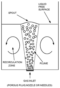Figure 3. Typical experimental set-up

Concerning the gas velocity, three zones can be identified (for example Castillejos and Brimacombe 1987): in the region close to the injection point there is a steep gradient in bubble velocity radially, and the motion of the bubbles is strongly affected by the gas injection velocity and mode of injection; in the fully-developed flow region, the mean bubble velocity, and the standard deviation of the bubble velocity spectrum, exhibit relatively flat radial profiles, and the bubbles affect the flow only through buoyancy; close to the liquid surface, the axial bubble velocity decreases more rapidly as liquid begins to flow radially outwards from the plume. The same change in bubble behaviour near the inlet was observed by (Anagbo and Brimacombe 1990) for injection through a porous plug. The slip velocity between the bubbles and the liquid is well represented by the terminal rising velocity of the same size bubble in stagnant liquid, as has been found also by (Sheng and Irons 1995).

Concerning the turbulence properties, some experiments (Johansen et al., 1988, Gross and Kuhlman, 1992, Iguchi et al., 1995, Sheng and Irons, 1993, Grevet et al., 1982), show a general isotropy of turbulence, while anisotropy (in the direction of gas-motion) is observed in the plume and near the walls by (Grevet et. al., 1982). Iguchi et al., 1995, found the turbulent velocities to be of the same order of magnitude as the mean velocities, and to be Gaussian-distributed. In the experiments of (Johansen et. al., 1988), the axial turbulent component is close to half of the corresponding mean velocity, and is greater than the radial one, except near the surface. Only in the experiment of (Gross and Kuhlman 1992) is the radial component larger (almost double) than the axial component, while (Sheng and Irons, 1993), found that the two components are approximately equal.

Later on, (Hassan 2002, 2003, 2006, 2011, 2012, 2013, Hassan and Tamer 2006, Abdulmouti, et. al. 2000, Hassan et. al. 1997, 1998, 1999- No. 1, 1999- No. 2 and 2001, Hassan and Esam, 2013) addressed details studies on the following research subjects:

1- The detailed flow structure and the global flow pattern of bubbly two-phase flows. And the fluid dynamic characteristics of a bubble plume, especially focusing on the technique for generating and using a strong and high speed surface flows at a free surface by using a bubble plume in order to improve the applications of the bubble plume and to collect surface-floating substances especially an oil layer during large oil-leakage accidents in order to protect naval systems, rivers, and lakes. Here is a summary of their results on these topics:

A- There are two large circulation flow regions of liquid near the bubble plume (at the right and the left side of the bubble plume).

B- The local liquid flow pattern around the bubble plume depends on the gas flow rate. It is recognized that as the gas flow rate increases, the magnitude of velocity increases and the effective area of the bubble plume (the width of the surface flow) expands in the horizontal direction.

C- Inside the bubble plume and near the free surface, the velocity of the two-phase flow is higher while it is slower in other regions. Hence, high speed two-phase flow is maintained and further accelerated along the vertical axis, and it produces large entrainment flow in the lower region. This is due to the effect of the buoyancy of bubbles. Hence, the generation of this high speed flow is considered a main contribution to induce a strong surface flow. If a vertically rising liquid jet is applied to induce the surface flow instead of the bubble plume, the high speed upward flow is not maintained near the free surface due to the turbulent momentum dissipation and the lack of the buoyancy inside the jet, and in this case the power efficiency is considerably less due to the dissipation of momentum under the free surface.

D- The spacing of the streamlines becomes smallest at the free surface. Moreover, near the free surface, the liquid flow in the horizontal direction is maintained over long distances. Hence, the maximum velocity in the horizontal direction is observed to be near the free surface. This means that the horizontal velocity is fastest on the free surface since there is no shear stress acting on the free surface. This is also one of the reasons why such a wide and thin surface flow is generated by the bubble plume.

E- The highest kinetic energy is generated at a long distance (far up) inside the bubble plume and in the vicinity of the free surface. This observation confirms the fact that the bubble plume can indeed generate a strong and wide surface flow over the bubble generation system.

F- The results of the whole flow field structure obtained by the PIV measurement show good analogy with those obtained by the numerical prediction.

2- Separation of bubbles and tracer particles by processing the original images, by using an image processing software in order to measure the velocity distribution of both gas and liquid phases in a bubble plume. In addition, to get information and knowledge of the relative velocity which is important to study the response of bubbles and that of the ambient (surrounding liquid). Since a simultaneous measurement of the velocities of both bubbles and liquid demands a separation of bubble images and tracer images in the same frame. This step was very important in order to study and clarify the flow pattern for both bubble motion and particle motion (liquid).

3- The fundamental characteristics (fundamental features) of the surface flow generation mechanism induced by the bubble plume, in spit of the complexity and irregularity (respectively nonlinearity) of the surface flow behavior near a free surface due to the strong dynamic interaction between the bubble and vortex motion. Moreover, detailed discussion concerning the actual surface flow generation process, which depends on the gas flow rate, the bubble size, and the internal two-phase flow structure of the bubble plume in the vicinity of the surface. In addition, the dependence of the surface flow speed on bubble’s injection condition. Hence, it made a room for more improvement toward higher efficiency in generating the surface flow. Their results showed that the maximum surface velocity increases with the gas flow rate at a power index of around 0.25 to 0.45. The increase of the surface flow velocity responds to the increase of liquid volume flux pumped by the bubbles. Moreover, the power index of the bubble diameter for the surface flow velocity ranges from -0.75 to -0.25. Their results indicated that the smaller the bubbles the faster the induced surface flow velocity. Moreover, the local fluctuation velocity increases with increasing gas flow rate. It concentrates, however, in the bubble plume region and close to the end wall. The fluctuations calm down in the region where the surface flow is fast. This inverse relationship is considered as one of the factors stabilizing a high speed and thin surface flow and it elucidates the reason why the surface flow is maintained over long distances. Moreover, their results indicated also that when a bubble plume reaches the free surface, the liquid phase flow changes its orientation rapidly from the vertical to the horizontal direction in the vicinity of the free surface. Therefore, the rapid distortion of the liquid phase results just in a layer under the free surface. Moreover, high vorticity distribution, high shear strain rate and high shear stress rate are generated by the surface flow. These phenomena appear in the layer under the free surface. Therefore, it can be said that the initial surface flow is rapidly generated in this layer. This is qualitatively different from (not found in) the case of a single-phase liquid jet flow whose speed is equivalent to the bubble plume. Hence, a surface flow is more effectively generated by means of bubbles than by a liquid jet flow because the distortion point appears in the vicinity of surface. On the other hand, the width of the upward flow induced by the bubble plume is larger than the thickness of the surface flow.

4- The transportation effect of surface floating substances due to a bubble plume is qualitatively confirmed by flow visualization using floating particles. As a result, it is confirmed that when the bubble plume is utilized, surface floating substances (which are the floating particles in their experiments) do not reach and/or do not stick on the oil fence (which is the cylinder in their experiments). Furthermore, the waves become extinct and damped. This is because the elliptical fluid motion of the wave vanishes due to the appearance of the strong surface flow induced by the bubble buoyancy close to the cylinder. In addition, the decrease of the average local density and the turbulence generation due to the inclusion of bubbles are important factors, which reduce the local kinematic energy of the wave near the cylinder. Moreover, the combination of the cylinder and the bubble plume gives us the highest safety for the prevention of these surface floating substances from crossing the cylinder position. Hence, the surface flow induced by the bubble plume is quite useful to control the surface floating substances and the bubble plume can stop the spreading of the surface floating substance.

5- Several experiments with many different situations were carried out to identify the effect of a bubble plume. The efficient effect of wave damping due to the bubble plume generated surface flow is confirmed. It becomes especially remarkable for waves with short wavelengths. The following conclusions can be drawn and summarized:

A- The bubble plume reveals a remarkable effect on wave damping due to the surface flow (which depends on the bubble generation condition). It is a very effective tool to decrease the wave parameters and extinct the wave motion on the free surface.

B- The wave damping effect is much greater for the bubbling case than for the non-bubbling case. The effect of the wave damping with bubbles is 3.3 to 8.8 times greater than without bubbles.

C- In case of using the bubble plume as an oil fence application, the effect of the bubble plume is much larger than that in case of using only a conventional oil fence. The present results confirm that the bubble plume is very useful and workers on the coast expect to work with more ease.

Moreover, Flow visualization of the bubble plume in two immiscible stratified fluids is carried out by (Hassan 2002, 2003, 2006, 2011, 2012, 2013) in order to improve the applicability of the bubble plume as an oil fence. Figure 4 shows samples of his recorded images of the flow field around a bubble plume and for a range (many cases) of gas flow rates. The pathlines are calculated as shown in Figure 5. The covering effect of the oil layer on the free surface and the influence of the convection due to the bubble plume are investigated by using image processing and PIV measurements. The main results are summarized as follows:

1- The PIV measurements and the pathlines measurement results of the internal flow structure of immiscible two-phase stratified liquids show that the velocity of the surface flow induced by the bubble plume in the vicinity of the oil-water interface is larger and stronger than that inside the oil layer. Moreover, the surface flow is particularly rapidly generated in the vicinity of the oil-water interface. It is confirmed by the their research that the flow structure is sensitively modulated by the gas flow rate. The main results explore the following points:

A- There are two circulating flows of liquid near the bubble plume for both the water and the oil layers. The flow circulations inside the water layer are larger than that inside the oil layer.

B- The velocity of the liquid is high inside the bubble plume, in the water layer, and near the oil-water interface, but low in other regions.

C- It is recognized that as the gas flow rate increases, the magnitude of the velocity increases and the effective area of the bubble plume (the width of the surface flow) expands in the horizontal direction. Two effective areas could be recognized: the first one is located at the oil-water interface and the second is located on the free surface. Hence, the surface flow of the oil-water interface, which is induced by the bubble plume, is stronger and larger than that induced in the free surface over the oil layer.

D- For large gas flow rate values a strong vortex motion (turbulent motion) is induced inside the deformed area. This vortex motion has a role in generating strong shear stress near the oil-water interface.

E- The highest kinetic energy is generated at a long distance inside the bubble plume and in the vicinity of the oil-water interface. This observation confirms the fact that the bubble plume can indeed generate a strong and wide surface flow over the bubble generation system.

2- The oil layer is easily broken by bubbles. It is confirmed that the oil stratum can be separated by a bubble plume especially when the bubble plume has high void fraction and high gas flow rates.

3- The altitude Δh of the upheaval bulge of the two-phase stratified liquid interface which is induced by the bubble plume (which plays an important role in breaking and destroying the oil layer) is measured experimentally and calculated theoretically. The experimental results agree up to a certain limit with the theoretical result.

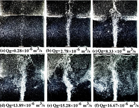Figure 4. Samples of the recorded images at various gas volume flow rates

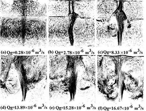Figure 5. The pathlines of the flow pattern at various gas volume flow rates

On the other hand, Simple plume models have been considered in various contexts. (Morton et al. 1956) used a simple plume model in their paper introducing the entrainment hypothesis; (Milgram 1983) compared his experimental results with the values predicted by a simple plume model, whereas (W¨uest et al. 1992) used both a simple plume model with the entrainment hypothesis to describe the effect of dissolving plumes. The work of (Brevik 1977) is also based on a simple plume formulation, though without making use of the entrainment hypothesis. (McDougall 1978) modelled the system as an inner circular plume containing the gas bubbles and some entrainment water, and an annular plume containing only water. The formalism of McDougall was generalized by (Asaeda and Imberger 1993, and Crounse et al. 2007), simplifying the implementation of density effects of dissolving bubbles. An extensive comparison between mixed and two-fluid models based on the entrainment hypothesis is given by (Bhaumik 2005). The advantages of the integral models are that the governing equations allow insight into the flow dynamics; they are computationally efficient and produce reasonable results in many cases. A drawback is that the integral models lose their validity, as the plume becomes less self-similar (Socolofsky et al, 2002), the kinetic energy approach to buoyant plumes of (Brevik 1977 and Brevik and Killie 1996) is generalized in order to allow for dissolution of gas. The model is compared to experiments carried out by (Milgram 1983) and is found to reproduce experimental data with satisfactory accuracy. The results presented suggest that the model presented yields a good starting point for the description of the dynamics and dissolution of gas in the zone of established flow for an air-bubble plume, given that the turbulent correlation parameter (I) is chosen correctly (Kristian and Iver 2008).

The detailed investigation of an unstable meandering bubble plume created in a 2-mdiameter vessel with a water depth of 1.5m is reported for void fractions up to 4% and bubble size of the order of 2.5 mm. Simultaneous PIV measurements of bubble and liquid velocities and video recordings of the projection of the plume on two vertical perpendicular planes were produced in order to characterize the state of the plume by the location of its centreline and its equivalent diameter. The data were conditionally ensemble averaged using only PIV sets corresponding to plume states in a range as narrow as possible, separating the small-scale fluctuations of the flow from the large-scale motions, namely plume meandering and instantaneous cross-sectional area fluctuations. Meandering produces an apparent spreading of the average plume velocity and void fraction profiles that were shown to remain selfsimilar in the instantaneous plume cross-section. Differences between the true local time-average relative velocities and the difference of the averaged phase velocities were measured; the complex variation of the relative velocity was explained by the effects of passing vortices and by the fact that the bubbles do not reach an equilibrium velocity as they migrate radially, producing momentum exchanges between high- and low-velocity regions. Local entrainment effects decrease with larger plume diameters, contradicting the classical dependence of entrainment on the time-averaged plume diameter. Small plume diameters tend to trigger ‘entrainment eddies’ that promote the inward-flow motion. The global turbulent kinetic energy was found to be dominated by the vertical stresses. Conditional averages according to the plume diameter showed that the large-scale motions did not affect the instantaneous turbulent kinetic energy distribution in the plume, suggesting that large scales and small scales are not correlated. With conditional averaging, meandering was a minor effect on the global kinetic energy and the Reynolds stresses. In contrast, plume diameter fluctuations produce a substantial effect on these quantities (Marco et. al. 2009).

In fact, older studies of bubble plumes (e.g. by Kobus 1968 and Milgram 1983) produced the basic understanding about their global behaviour. More recent detailed bubbly flow experiments (Hassan et al. 1992, Delnoj et al. 1999, Kubasch 2001 Rensen and Roig 2001, Simiano et al. 2006) were conducted with confined flows or bubble columns. Various effects including recirculation in the vessel and the presence of walls can make the plume centreline and boundaries oscillate in three dimensions. These effects can also produce large structures driving the dispersed phase. The three-dimensionality of air–water bubbly flows was revealed in various experiments; (Milgram 1983, Castello-Branco and Schwerdtfeger 1994, Kuwagi and Ozoe 1999 and Johansen et al. 1988) discuss plume precession and swirling. The radial distributions of the void fraction and of the velocities were investigated by several authors, e.g. (Tacke et al. 1985 and Johansen et al. 1988).

Turbulence in bubbly flows has been central to the research in this area. Experiments of (Johansen et al. 1988, Gross and Kuhlman 1992 and Iguchi et al. 1995) revealed that turbulence is in general isotropic in the core flow, whereas anisotropy was shown to take place only near the walls by (Grevet, Szekely and El-Kaddahn 1981). This was to be expected indeed, but more detailed description of the exact role of the gas phase in producing anisotropy of turbulence and its proportions was given later by other authors. (Iguchi et. al. 1991) found that the velocity fluctuations may be of the same order of magnitude as the mean velocities (100% turbulence intensities), and follow a Gaussian distribution. In the experiments of (Johansen et al. 1988), measured turbulent intensities were weaker axially than in the experiment of (Iguchi et al. 1991), i.e. about 50%, but still substantially stronger in the radial direction (>100 %) except near the free surface. A fairly exhaustive literature survey on bubbly plumes can be found in (Simiano 2005). (Simiano et al. 2006) have listed the main Publications and presented a comprehensive investigation of the most important hydrodynamic characteristics of fairly large-scale bubble plumes. Their plumes, produced in a 2-m diameter vessel with a 0.3-m diameter circular bubble injector, exhibited the usual meandering behaviour. In addition, the shape and dimensions of the plume cross-section varied in time and the structure of the plume showed the typical unstable behaviour recently reported, for example, by (Rensen and Roig 2001). As one of the goals of the (Simiano et al. 2006) study was to determine the turbulent characteristics of the plume and study the fluctuating components of the main flow variables, it became evident that the usual averages of the data (or referred as ‘global averages’), produced with an unstable plume were not at all representative of any instantaneous plume condition. The meandering and instabilities of the plume were indeed ‘spreading’ the profiles of the variables of interest and the local fluctuations obtained via global averaging of the data were affected by the macroscopic instabilities of the plume. It also became clear that attempts to ‘stabilize’ the plume were questionable and would had affected its behaviour. A much more promising way would have been to study the characteristics of the plume making use of conditional ensemble averages according to its instantaneous state.

In addition, turbulent bubbly flows in vertical pipes or channels are frequently encountered in industrial systems, such as power plants, nuclear reactors, food production, chemical process facilities, and wastewater treatment plants. The interaction of the dispersed bubbles and the continuous fluid has a great effect on the efficiency and safety of these operations. To better understand the dynamics of these flows, a number of investigations have been done in the past. (Oshinowo and Charles 1974, Serizawa et. al. 1975, Nakoryakov et. al. 1981, Wang et. al. 1987, Liu and Bankoff 1993, Nakoryakov et al. 1996, Kashinsky and Randin 1999 and Sun et. al. 2004). These authors carried out experiments to measure not only the void fraction distribution and the liquid velocity profile, but also the turbulence structure across the pipes and channels. Many analytical and computational studies have also been performed to predict the liquid turbulent structure in bubbly flows. (Bankoff 1960) was one of the first to analyze the lateral void fraction distribution for a bubbly flow. Subsequently, many predictions based on the mixing-length model, (Levy 1963 and Beattie 1972) the driftflux model, (Clark and Flemmer 1985) and the two-fluid model (Drew and Lahey 1979 and 1982, Lopez et. al. 1994, Politano et. al. 2003, Guet et.al. 2005) have been carried out.

On the contrary, most of the investigations considered the cases of upward bubbly flows. Only a few investigations have been performed for downward flows, although a good understanding of the downward two-phase flow is indispensable for advanced nuclear reactor design and safety analysis. (Ishii et. al. 2004 and Oshinowo and Charles 1974) were among the first to study downward gas-liquid flows in vertical tubes. They found that the gas velocity in downward flow was always less than in upflow. Later, (Clark and Flemmer 1985 and Clark and Flemmer 1984) experimentally studied the averaged bubble velocity for downward bubbly flows in vertical pipes and used the drift flux model to correlate the experimental data. (Wang et al. 1987 and Kashinsky and Randin 1999) carried out detailed experiments to measure the local liquid velocity profiles and the turbulence structure in bubbly downflow. Recently, a series of experiments for downward two-phase flow were performed by Ishii and co-workers. (Ishii et. al. 2004, Hibiki et. al. 2004 and Sun et. al. 2004) measured the local liquid velocity and phase distribution of the vertical downward two-phase flow, with a primary focus on the interfacial area transport mechanism. These studies show that the bubbles accumulate in the core region of pipes or channels, and the phase distribution and velocity profile are quite different from those of upward bubbly flow.

Moreover, The simulations of (Lu, Biswas, and Tryggvason 2006) to buoyant bubbles in a turbulent down-ward flow were extend by (Jiacai and Gretar 2006) and study the effect of the average void fraction on the phase distribution, the velocity profile, and the flow characteristics.

Direct numerical simulations are used to study turbulent bubbly downflows in a vertical channel by (Jiacai and Gretar 2006). All flow scales, including the bubbles and the flow around them, are fully resolved using a front-tracking/finite-volume method. The turbulent bubbly channel flow is driven downward by an imposed constant pressure gradient, and the friction Reynolds number of the flow, based on the friction velocity and half-width of the channel, is 127.3, corresponding to a bulk Reynolds number of 3786 for a flow without bubbles. Three cases with several nearly spherical bubbles are examined. The bubble diameter is 31.8 wall units for all cases but the number of bubbles is varied, giving average void fractions of 1.5%, 3%, and 6%. The lift force on the bubbles drives them away from the walls until the mixture in the center of the channel is in hydrostatic equilibrium. Thus, the flow consists of a core region where the average void fraction and the mean vertical velocity are approximately constant and a bubble-free wall layer. The vertical velocity fluctuations in the wall layer decrease as the void fraction increases and the width of the wall layer decreases, but in the bubble-rich core the velocity fluctuations are higher than for a corresponding single-phase turbulent flow (Jiacai and Gretar 2006).

In turbulent water flows, large quantities of air bubbles are entrained at the free-surfaces. Practical applications of gas-liquid bubbly flows are found in Chemical, Civil, Environmental, Mechanical, Mining and Nuclear Engineering. Air-water flows are observed in small-scale as well as large-scale flow situations. Typical examples include thin circular jets used as mixing devices in chemical plants (Q_w ~ 0.001 L/s, diameter ~ 1 mm) and spillway flows (Q_w > 10,000 m³/s, flow thickness over 10 m). In each case, however, the interactions between the entrained air bubbles and the turbulence field are significant.

(Hubert 1999) work aims to gain a better understanding of the basic mechanisms of gas entrainment and the interactions between entrained gas bubbles and the turbulence. He presented new analysis and experimental results, to compare these with existing data, and to present new compelling conclusions regarding momentum and void fraction development of air-water gas-liquid bubbly flows.

(Hubert 1999) presented a comprehensive analysis of the air entrainment processes in free-surface turbulent flows. The air-water flows are investigated as homogeneous mixtures with variable density. The variations of fluid density result from the non-uniform air bubble distributions and the turbulent diffusion process. Several types of air-water free-surface flows are studied: plunging jet flows, open channel flows, and turbulent water jets discharging into air (Hubert 1999).

Beyond that, air bubble systems have been used extensively and for a variety of purposes such as, pneumatic breakwaters, prevention of ice formation, as barriers against salt water intrusion in rivers and locks, for stopping the spreading of oil spills on the water surface, for reduction of underwater explosion waves and for agitation and mixing operations in process industries. However, the technique may also be used for destratification and water quality control Management of lakes and, reservoirs in which case the characteristics of the air-bubble plume are of more interest than the induced horizontal flow in the surface layer (Klas and John 1970).

The air flow discharged into water rapidly expands, due to the pres sure drop acros s the nozzle, and breaks up into bubbles of discrete size. This initial formation of the gas bubbles has been studied both theoretically and experimentally, see for instance, (Davidson and SchUler 1960). Several studies on the motion of gas bubbles in liquid are reported in the literature. (Haberman and Morton 1954) carried out a comprehensive investigation on the rise velocity of single air bubbles in still water (Klas and John 1970).

In fact, the similarity between the air-bubble plume and a simple buoyant plume was first pointed out by (Taylor 1955) in a discussion on the use of pneumatic breakwaters. (Bulson 1962) derived semiempirical relations for maximum velocity and thicknes s of the layer of horizontal surface flow. (Sjoberg 1967 and Kobus 1968) have studied the flow induced by air-bubble systems both experimentally and theoretically using the similarity to jet and plume mixing.

Furthermore, the air bubble plume induced by the steady release of air into water has been analyzed with an integral technique based on the equations for conservation of mass, momentum and buoyancy. This approach has been widely used to study the behavior of submerged turbulent jets and plumes. The case of air-bubble induced flow, however, includes additional features. The compressibility of the air and the differential velocity between the rising air bubbles, and the water were introduced by (Klas and John 1970) as basic properties of the air bubble plume in addition to a fundamental coefficient of entrainment and a turbulent Schmidt number characterizing the lateral spreading of the air bubbles. Theoretical solutions for two- and three-dimensional air-bubble systems in homogeneous, stagnant water were presented in both dimensional and normalized form and compared to existing experimental data. The further complication of a stratified environment was briefly discussed since this case is of great practical interest. The theory was compared to the experimental data reported by (Kobus 1968 and Klas and John 1970).

Complex, 3D mixing of single- and multi-phase flows, in particular by injection of gas and creation of bubble plumes, occurs in a number of situations of interest in energy technology, process and environmental engineering, etc. For all these applications, the basic need is to determine the behaviour of the bubble plume and the currents induced by the ascending gas plume in the surrounding liquid and thereby the consequent mixing in the body of the liquid (Massimo 2002).

A six-equation, two-fluid model was utilized by (Massimo 2002) and transient calculations were performed to study the plume growth, the acceleration of the liquid due to viscous drag, and the approach to steady-state conditions. All calculations were performed using the commercial CFD code CFX4, with appropriate modifications and code extensions to describe the interphase momentum forces and the turbulent exchanges between the phases. Since the k-ε is a single-phase model, an extended version was used, with extra source terms introduced to account for the interaction between the bubbles and the liquid. A new model was advanced to relate turbulent bubble dispersion to statistical fluctuations in the liquid velocity field, affecting the drag and lift forces between the phases. The model is able to account for the dispersion of bubbles due to the random influence of the turbulent eddies in the liquid, such as the empirical Turbulent Dispersion Force, and has the advantage that no fitting coefficients need to be introduced (Massimo 2002).

The interphase forces are not the only source of empiricism: the above-mentioned extra source terms introduced into the k-ε model, are patch-ups which introduce ad hoc empirical coefficients which can be tuned to get good comparison with the data. Further, the hypothesis of turbulence isotropy has still to be rigorously proved with clean experimental data. The Reynolds Stress Models (RSMs), which are in principle appropriate for this kind of flow (since equations are solved for each component of the Reynolds stress tensor), are unstable and not robust enough, and it is difficult to achieve convergence even for single-phase flows. Therefore, attention was focused on Large Eddy Simulation (LES) turbulence models (Massimo 2002).

The main advantage of LES for this class of flows is that it captures directly the interactions of the bubbles with the resolved large-scale structures up to the size of the grid (close to the bubble diameter), whereas the interaction with the subgrid scales can be modelled. In other words, the turbulent dispersion of the bubbles is due only to the largest structures, which are calculated directly with LES. Since this is a new area of study, many open questions need to be addressed: a universally-accepted, two-phase subgrid model does not exist, and the influence of the grid on the simulation is also not clear, since this determines the scales that are going to be resolved. To pursue this approach, the LES model was implemented into CFX-4. First, a single-phase test case has been calculated to validate the model against the data of (George et. al., 1977). Second, a simple case (a 3D box with homogeneous distribution of bubbles) has been run to study the modifications induced by the bubbles on the turbulence of the system and the effect of the filter (mesh size). The results have been obtained with the (Smagorinsky 1963) subgrid model and were compared with the experimental data of (Lance and Bataille 1991), finding that the turbulence intensities increase with the mesh size, and the optimum configuration requires a mesh comparable to the bubble diameter; otherwise the liquid velocity fluctuations profile is not captured at all, meaning that the grid is too coarse. The idea recalls the Scale-Similarity Principle of (Bardina et al., 1980).

Taking advantage of this experience, two more elaborate situations, closer to reality, were analyzed: the case of a turbulent bubbly shear flow in a plane vertical mixing layer, with calculations compared against the data of (Roig, 1993); and the case of the bubble plume, with calculations compared against the data of (Anagbo and Brimacombe, 1990). A study on the importance of the lift force has been carried out and the results were similar in both cases, with an optimum lift coefficient of 0.25. The results showed good agreement with the experiment, although a more detailed study of bubble-induced turbulence (or pseudoturbulence) is required. The (Germano et al., 1991) dynamic procedure was successfully tested and a new subgrid scale model for the dispersed phase that requires no empirical constants, was introduced (Massimo 2002).

10. Conclusions

As a result, it is clear that the bubble plume “which is a typical bubble flow” is a key phenomenon to be studied and investigated, and it is an effective tool for many applications and can indeed contribute to various improvements. The motivation to study the bubble plume is the demands to improve its performance and its applications. Especially in many engineering fields as materials, chemical, mechanical, modern industrial technologies, and in the environment in order to protect the natural environment, the naval planets, navel systems, rivers, lakes, etc from pollution. Hence these engineering fields are expected to benefit from the improvement and development of the bubble plume.

The present work demonstrates, reviews and summarizes the major finding of previous research of the following points:

1) The techniques and the important models for the measurement of the dominated two-phase bubbly flow/ bubble plume parameters such as flow regime, bubble size and shape, bubble velocity and void fraction which are considerably important and play an important role in operational safety, process control and reliability of continuum processes of many engineering applications.

2) Turbulent bubbly flow structure.

3) Some important applications especially on bubbly two-phase flow/bubble plume and its associated surface flow since it can contribute to improvements in various directions.