1. Introduction

In every circumstances where combustion occurs, the formation of Nitrogen Oxides (NO_x) are unavoidable. From a home open fire to a coal fired power plant, NO_x is formed as an undesired product and a contributor to air pollution and health problems. Due to the increasing concerns over the environmental pollution, the understanding of the NO_x formation mechanism during the combustion process and of the development of their reduction technologies is essential for the efficient design of combustion devices. But, one of the great challenges in predicting the formation of the NO_x in a combustion process is the chemical time-scale, which is slow.

NO_x is used to refer to the nitric oxide NO and the nitrogen oxide NO₂. Typically 95% of the total NO_x emissions is nitric oxide, NO, which is the primary form in combustion products. The nitric oxide NO is subsequently oxidized to NO₂ in the atmosphere.

There are four different routes or mechanisms in the formation of NO_x, which were identified by Bowman [2]. These are the thermal NO route, the prompt NO route, the N₂O (nitrous oxide) route, and the fuel-bound nitrogen route.

But, it is known that in nonpremixed combustion of hydrocarbon fuels, the first two mechanisms dominate the process of nitric oxide, NO, formation. The thermal NO also well-known as the Zeldovich NO proposed by Zeldovich [3], which dominantly depends on its local temperature and reactants (O₂ and N₂). The prompt or Fenimore NO mechanism proposed by Fenimore [4], is formed through hydro-carbon radical reaction with molecular nitrogen under fuel-rich condition. In most flames, especially those from nitrogen-containing fuels, the prompt mechanism is responsible for only a small fraction of the total NO_x.

Meunier et al. [5] investigated the NO_x emissions from turbulent propane diffusion flames experimentally as well as numerically. In numerical investigation both the thermal and prompt NO reaction mechanism were used to predict NO formation. The equations were closed by k-ϵ turbulence model where as the combustion was modelled using the stretched laminar flamelet model and the probability density function (PDF) method.

Formation characteristics of the nitric oxide in a three-stage air/LPG flame has been investigated both experimentally and numerically by Kim et al. [6] including both the thermal and the prompt NO formation mechanism through a conservation equation of NO mass fraction. The computed results were compared with the experimental measurements.

For the hydrogen jet diffusion flame, a prediction method for NO applicable to LES was presented by Taniguchi et al. [7]. To model NO production, they considered the extended Zeldovich mechanism with the quasi-steady state approximation of the nitric atom through the balance equation of NO mass fraction. In LES, they neglected the SGS contribution to the NO production.

Modeling of radiation and NO formation in turbulent nonpremixed flames using a flamelet/progress variable formulation has been investigated by Ihme and Pitsch [8]. In NO production model, a transport equation for the NO mass fraction was considered, and they obtained the chemical source term from the flamelet library. The NO model formulation was analyzed separately for the thermal, nitrous oxide, and prompt NO reaction mechanisms.

Chun et al. [9] performed a numerical study on extinction and NO_x formation in nonpremixed flames with syngas fuel. Numerical simulations were done in a quasi-one dimensional counterflow configuration using the OPPDIF code adopting GRI-Mech 3.0 for the chemical reaction mechanism. They have considered a reaction path diagram to analyze NO_x formation pathways along with the thermal NO_x formation mechanism. They found that the NO production through the thermal mechanism was weakened more than that through the non-thermal mechanism, and most of the NO_x production started from the N₂ → NNH pathway.

In this paper LES technique has been applied to investigate the NO formation in the non-premixed propane-air turbulent combustion process within a cylindrical combustor. A schematic of computational domain is shown in Fig. 1. Gaseous propane (C₃H₈) is injected through a circular nozzle of an internal diameter of 2mm at the centre of the combustor inlet while the preheated air of temperature 773K with an averaged velocity of 0.96ms⁻¹ is supplied through the circular inlet of 115mm internal diameter into the 350mm long combustion chamber. The overall equivalence ratio is 0.6 so that burning occurs in a fuel-rich nonpremixed combustion mode, which produces various forms of hydrocarbons in the combustion products. The average fuel velocity measured by [1] at the inlet is 30ms⁻¹. A Smagorinsky model with C_s = 0.1 as well as its dynamic calibration has been employed to model the sub-grid scale stresses, while the non-premixed combustion process is modelled through the conserved scalar approach with laminar flamelet model. The NO production mechanism is modelled through a balance equation for NO mass fraction. The extended Zeldovich (thermal) reaction mechanism is taken into account to model the NO production.

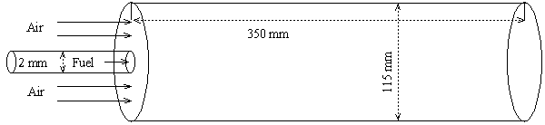Figure 1. A schematic of the cylindrical combustor with short computational domain

This paper is structured in the following order. The modelling of the NO formation is presented in §2, followed by the Mathematical formulation for LES including the sgs modelling and the conserved scalar approach to combustion modelling in §3. In §4 the numerical procedure and the necessary boundary conditions used in the LES are described. Results and discussion are presented in §5. In §6 a general conclusion of this paper is made.

2. Nitric Oxide (NO) Prediction Model

In a non-premixed combustion process a high temperature is occurred at the stoichiometric interface where the thermal reaction mechanism of NO dominates its formation. So, the maximum flame temperature is the most important parameter that determines the potential for NO formation. The high NO levels that occur in practical systems can only be reduced by reducing the thermal NO formation. In the present NO formation model, the extended Zeldovich (thermal) reaction mechanism proposed by Zeldovich [3], is taken into account through the solution of a transport equation for NO mass fraction (see equation (8)). The extended Zeldovich reaction mechanism has the following three reactions;

(1)

(2)

(3)

According to the above reactions, the formation rate of NO is

(4)

and the rate for nitrogen atoms is

(5)

Assuming a quasi steady state assumption of the nitrogen atoms, i.e., d[N]/dt ≈ 0, , yields the rate of formation of NO as

(6)

where [N2] = ρY_N2/M_N2, [O] = ρY_O/M_O; M_N2 = 28 kg/kmol and M_O = 16 kg/kmol are the molar mass of N₂ and O respectively. The reaction rate, k₁, based on Baulch et al. [10, 11] is taken as

(7)

where R = 8.314472J.K−1.mol−1 is the universal gas constant.

The transport equation for NO is written as

(8)

where Y_NO is the mass fraction of NO.

The source term, ρS(Y_NO), for the formation of NO mass fraction per unit volume is therefore expressed as

(9)

where M_NO is the molecular weight of NO.

3. Mathematical Formulation for LES

In LES, a spatial filtering operation is applied to the governing equations of motions to separate the large scale (resolved scale) flow field from the small scale (sub-grid scale), Leonard [12]. Employing the density weighted Favre-filtered function, Favre [13] to the continuity equation, Navier- Stokes equations, the mixture fraction (conserved scalar) equation, and the conservation equation for NO mass fraction equation gives:

(10)

(11)

(12)

(13)

where t is time; x_j is any of the three coordinate directions; u_j is any of the three velocity components; p is the pressure; ρ is the density, which, in reacting flows, varies due to the heat release from the chemical reaction and on the chemical composition of the fluid. μ is the molecular viscosity, is the strain rate, δ_ij is the kronecker delta, ξ is the conserved scalar or mixture fraction and is the diffusion coefficient.

The instantaneous source term, , in conservation equation (13) for NO mass fraction is written as,

(14)

The NO production rate, r_NO, is a function of the flame temperature and the concentrations of N₂ and O (see equations (6) and (7)), which in turn can be expressed as a function of mixture fraction through the flamelet (Fig. 2) generated at a strain rate of 15s⁻¹. A details of reaction mechanism and the flamelet calculations can be found in Leung [14]. The flamelet temperature is adjusted to account for the radiative heat loss to the combustor walls by using the following relation, Fairweather et al. [15]:

(15)

where the radiative fraction, χ, is taken as 0.2, and T_ad represents the adiabatic flamelet temperature.

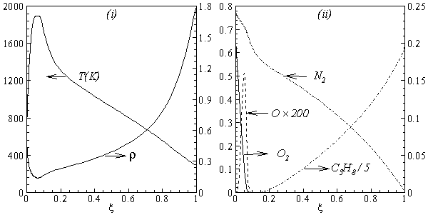Figure 2. Laminar flamelet calculation for strain rate of : dependance of (i) temparature and density; and (ii) mole fractions of C3H8, N2, O and O2, on the mixture fraction, ξ

The variation of the instantaneous NO production rate with the variation of the mixture fraction variance, ξ′², is presented in Fig. 3. This figure shows that the peak value of the the NO production rate decreases in magnitude and also shifts to larger values of the mixture fraction with the increasing values of ξ′². The Favre-averaged NO production rate, , for NO formation may therefore be determined by

(16)

where is the β-pdf (probability density function) constructed from predicted values of the conserved scalar, , and the sub-grid scalar variance, . Due to high peak appeared in NO production rate, it is convenient to use a piece-wise polynomial fitting approach (for details see, Paul [16]) for the best data fitting of the r_NO. Thus, a piece-wise polynomial fitting approach is used to integrate the β-pdf.

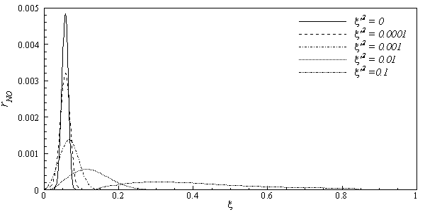Figure 3. Dependence of the instantaneous NO production rate on the mixture fraction and mixture fraction variances

The most famous and still widely used model for the subgrid scale stress is that of the Smagorinsky model [17]. The model is based on an eddy viscosity assumption and of the form of

(17)

where Δ is the filter width and is the magnitude of the large scale strain rate tensor, . Two computations have been performed, one with C_s = 0.1 (Case1) and another one with its dynamically calibrated values (Case2), proposed by Germano et al. [18].

For the subgrid scale scalar fluxes, , a gradient model, proposed by Schmidt and Schumann [19], of the form

(18)

is applied, where is a constant sub-grid scale Prandtl/Schmidt number which is assigned a value of 0.7.

In the NO model, we have used the same gradient model of Schmidt and Schumann [19] for modelling the subgrid scale NO mass fraction fluxes, .

The conserved scalar modelling approach with the laminar flamelet model, Peters [20], is applied to model the combustion. In this approach, it is assumed that the chemical reaction rates are fast compared to the rate at which the reactants mix. The mixing process is described by a conserved scalar which is also known as the mixture fraction. It is then considered that the instantaneous species concentrations are a unique function of this mixture fraction. Since this functional dependence is highly nonlinear, the mean or filtered values are obtained via the probability density function of the mixture fraction, Bilger [21]. The filtered density () and density weighted thermochemical variables () are obtained by integrating over a β - probability density function, once the density weighted mixture fraction, , and its sub-grid scale variance are known. Further details of this model are found in Paul [16], Paul et al. [22] and di Mare et al. [23].

4. Numerical Procedure

For the present simulation, a curvilinear body fitted coordinate system is employed. Inside the combustion chamber the grid consisting of a total of about 1.5 million nodes with a non-uniform mesh distributed along the three co-ordinate directions. As the fuel is injected through a circular nozzle at centre of the combustor inlet at a speed relatively higher than that of the air supplied through the cylinder, a steep gradient appears in this area. To resolve this steep gradient adequately a very fine mesh is required at the centre of the combustor. The mesh lines are contracted at the centre and the inlet of the combustor, and they are expanded smoothly in all the three directions outwards from the centerline and inlet.

The numerical solution procedure is based on the finite volume approach where the governing equations are integrated over the mesh control volume. The finite volume based in-house developed code LES-BOFFIN (Boundary Fitted Flow Integrator) has been used to solve the governing equations. The code is second order accurate in both space and time. The BOFFIN code has been applied extensively in the LES of reacting and non-reacting turbulent flows; for examples, see LES of a turbulent non-premixed propane-ar reacting flame, Paul et al. [22], of a gas turbine combustor, di Mare et al. [23] and of a turbulent nonpremixed flame, Branley and Jones [24]. Details of the numerical method used in the BOFFIN are not presented here for brevity.

In the simulation fully-developed turbulent pipe flow profiles were applied as the instantaneous inflow boundary conditions at the fuel nozzle, while a uniform velocity profile is applied for the air flow. The mixture fraction at the inlet is defined as

(19)

The NO mass fraction are negligibly small at the inlet and set to zero. Fig. 3 clearly shows that the production rate of NO is zero at ξ = 0.0 and 1.0. At the outlet boundary, a non-reflective boundary condition is used, a condition sufficient to minimize the effects of the outlet boundary in the solutions. A thin viscous sub-layer develops adjacent to the walls of the combustor and a prohibitively fine mesh would be required to resolve this. To overcome this difficulty an equilibrium log-law condition is employed as a near wall condition at the surfaces of the combustor.

5. Results and Discussion

We present the computational results in this section. The average time step, dt, used in the computation is at the order of 10⁻⁶. The results presented here in the form of time mean which are defined as

(20)

where is the time dependent results of a total of N = 3 x 10⁵ time steps.

The results are obtained for two cases, Smagorinsky constant, C_s, of 0.1 (Case 1) and dynamically calibrated C_s (Case 2). The solid lines indicate Case 1 and the dashed lines represent Case 2.

5.1. Temperature and Species Mole Fractions

The results of temperature and species mole fractions, which are required as an input to the NO formation model, are presented here.

Computationally predicted mean temperature, , results along axial and radial direction at different cross sectional positions are compared against the experimental measurement done by Nishida and Mukohara [1] in Fig. 4. In Fig. 4(a), at the inlet the predicted mean axial temperature on the centerline is same as the injected fuel temperature. The flame temperature then starts increasing and achieves a maximum value of 1696K (Case1) and 1730K (Case2) at the outlet. The corresponding peak temperature in the experimental investigation was recorded as 1765K, so the computation slightly under predict the temperature at the outlet. But the peak level of the mean temperature is better predicted in Case2. Moreover, the experimental results show a concave like shape around y = 0.2m, which is not evident in the predictions where a slight over-prediction is evident in both the cases.

In Fig. 4(b-d), the radial distribution of the mean temperature shows that the peak value of the computed temperature is slightly under-predicted and moves towards the wall near the inlet (frames b, c), and the temperature at the centre shows slight over-prediction in both the Cases. But a slight under-prediction of the temperature occurs at the centre in the downstream (frames d), but a better prediction is found in Case 2. Comparing the computed temperature distributions with the experiment, it is found that the trend of increasing and decaying of the temperature in the radial direction is matched reasonably well with the experimental data. However, both quantitatively and qualitatively a very good agreement is achieved with experiment.

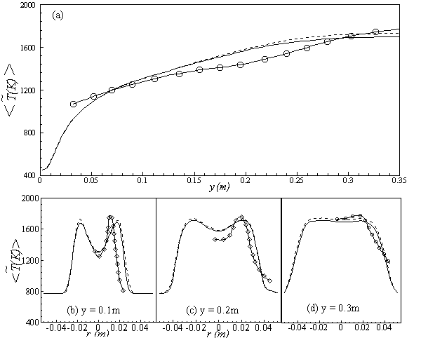Figure 4. Comparisons of the mean temperature, , with those of the experimental data along the (a) axial direction, and the radial direction at different cross-sectional positions: (b) y = 0:1m, (c) y = 0:2m and (d) y = 0.3m; Solid line, Case1; Dashed line, Case2; Solid line with circle, experimental

In Figs. 5-7, we present the results of the mole fraction of the three selected combustion species and comparisons with those of the experiment are made. Fig. 5(a) shows that the predicted axial mole fraction of the fuel has an excellent agreement with the experimental result. The mole fraction of the reactant in Fig. 5(b) is predicted well. While the in Fig. 5(c) is under-predicted at the downstream but predicted well against the experiment at the upstream. From the radial profiles for reactants , and in both locations at y = 0.1m (Fig. 6) and y = 0.3m (Fig. 7), we have a good agreement with the experiment. However, there are slightly over- and under- prediction at some positions but the trend is matched well with experimental measurements.

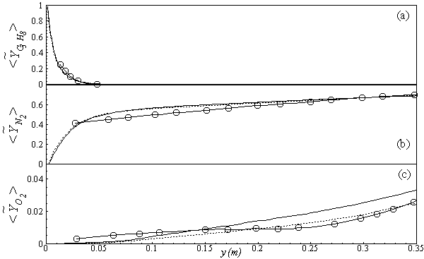Figure 5. Mean mole fractions: (a) , (b) and (c) along the axial direction; Solid line, Case1; Dashed line, Case2; Solid line with circle, experiment

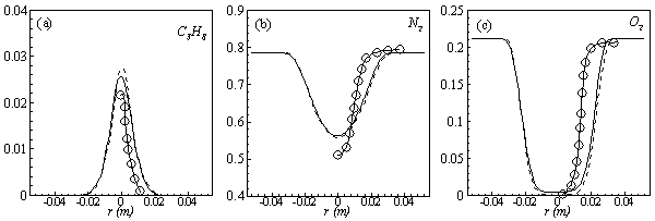Figure 6. Mean mole fractions: (a) , (b) and (c) along the radial direction at y = 0.1m; Solid line, Case1; Dashed line, Case2; Solid line with circle, experiment

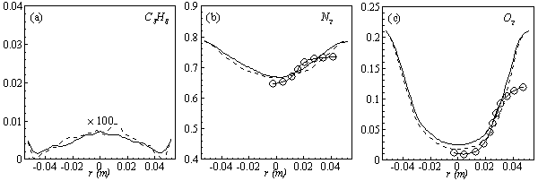Figure 7. Mean mole fractions: (a) , (b) and (c) along the radial direction at y = 0.3m; Solid line, Case1; Dashed line, Case2; Solid line with circle, experiment

5.2. Production Rate and Mass Fraction of NO

In Fig. 8 the time averaged results of the (a) temperature, , (b) NO production rate, , and (c) mass fraction of NO, , on the horizontal midplane of the combustor are plotted. The solid lines shown on the contour plots represent the locus of the stoichiometric mixture fraction. These contour plots, obtained in Case1, clearly show that the production of NO is highly dependent on both the flame temperature (frame (a)) and the concentration of N₂ (Fig. 5(b)). The mass fraction of NO reaches the maximum level at the stoichiometric zone.

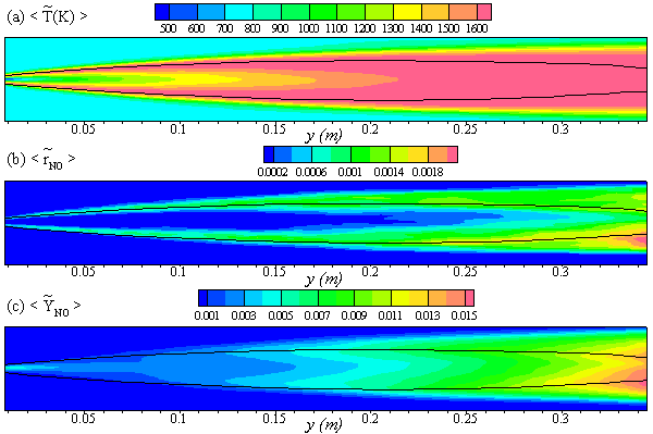Figure 8. The mean values of the (a) temperature, , (b) NO production rate, , and (c) NO mass fraction, on the horizontal mid-plane of the combustor, for Case 1

Mean axial and radial profiles of the NO production rate, , are depicted in Fig. 9. Axial profile on the centerline of the combustor, plotted in Fig. 9(a), shows that the rate is zero upto the axial distance y = 0.1, where the fuel stream dominates, afterwards the rate increases and gets its maximum at the outlet of the combustor. From the radial profile of the NO production rate, plotted in Fig. 9(b-d), it can be seen that the peak values are predicted in between the centerline and the combustor wall where the temperature (see Fig. 5(b-d)) as well as the concentration of N₂ (Fig. 6(b), 7(b)) has also its maximum, which can clearly be seen from the mean plot of the NO production rate presented in Fig. 8.

Predicted axial profile of the NO mass fraction (Fig. 10(a)) increases gradually as the flame temperature increases and achieves a peak level at the outlet of the combustor the maximum temperature (Fig. 4(a)) is recorded. This is simply because the present NO formation model includes the Zeldovich or thermal reaction mechanism in which the NO production rate is highly dependent on the temperature and reactants (N₂ and O₂). The radial profiles (Figs. 10(b-d)) of the NO mass fraction show that the NO production level decreases along the radial direction because of the temperature near the combustor wall which is very low although the N₂ level is predicted high in this region.

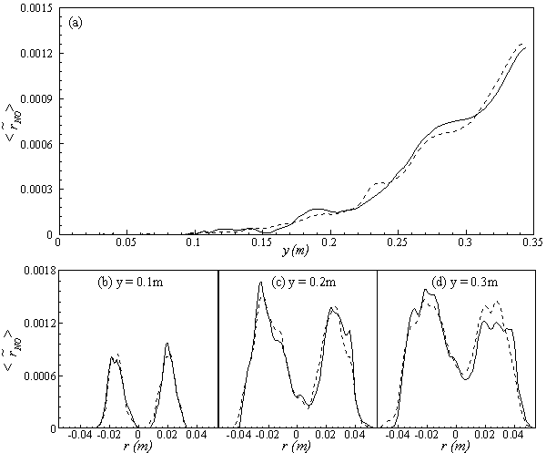Figure 9. Mean values of NO production rate, , along the (a) axial direction and radial direction at the different cross-section positions: (b) y = 0:1m, (c) y = 0:2m, (d) y = 0:3m of the combustor

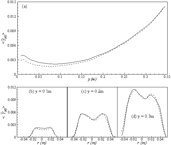Figure 10. Mean values of the NO mass fraction, , along the (a) axial direction and radial direction at the different cross-section positions: (b) y = 0:1m, (c) y = 0:2m, (d) y = 0:3m of the combustor

Comparison between Case 1 and Case 2 shows that Case 2 produces slightly low levels of the mean NO mass fraction in the upstream region, while towards the downstream both predictions gradually converge together.

6. Conclusions

Large Eddy Simulation technique has been applied to investigate the NO production in the non-premixed propane/air turbulent combustion process within a cylindrical combustor. In LES a constant valued Smagorinsky model as well as a dynamic model is taken into account for modelling the sub-grid scale stresses. The non-premixed combustion process is modelled through the conserved scalar approach with the laminar flamelet model, while the NO production mechanism is modelled through a balance equation for NO mass fraction. The extended Zeldovich (thermal) reaction mechanism is taken into account to model the NO production.

The computational results of temperature and selected species mole fractions have been compared with the experimental data obtained by Nishida and Mukohara [1] in the turbulent co-flowing propane and preheated air combustion, where a good agreement is achieved.

It was not possible to compare the computational results of the NO mass fraction with experimental data, as Nishida and Mukohara [1] did not perform any measurements on the NO mass fraction. However, the present results of NO clearly agree well with the principle and reaction mechanism of the extended Zeldovich (thermal) used for the modeling of NO. The NO mass fraction is predicted high in the high temperature zone.

The results are almost uninfluenced by the choice of sub-grid scale models although slightly lower prediction of NO mass fraction is found with dynamic Cs in the upstream. However, dynamic C_s produces a higher levels of the sub-grid scale quantities in the upstream region.