-
Paper Information
- Paper Submission
-
Journal Information
- About This Journal
- Editorial Board
- Current Issue
- Archive
- Author Guidelines
- Contact Us
American Journal of Fluid Dynamics
p-ISSN: 2168-4707 e-ISSN: 2168-4715
2014; 4(1): 6-15
doi:10.5923/j.ajfd.20140401.02
MHD Flow Analysis Using DTM-Pade’ and Numerical Methods
 Abstract
 Reference
 Full-Text PDF
 Full-text HTML
S. Baag1, M. R. Acharya2, G. C. Dash
1Department of Physics, College of Basic Science and Humanities, Orissa University of Agriculture and Technology, Bhubaneswar
2Department of Mathematics, Siksha ‘O’Anusandhan University, Bhubaneswar
Correspondence to: S. Baag, Department of Physics, College of Basic Science and Humanities, Orissa University of Agriculture and Technology, Bhubaneswar.
| Email: |  |
Copyright © 2014 Scientific & Academic Publishing. All Rights Reserved.
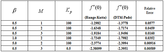
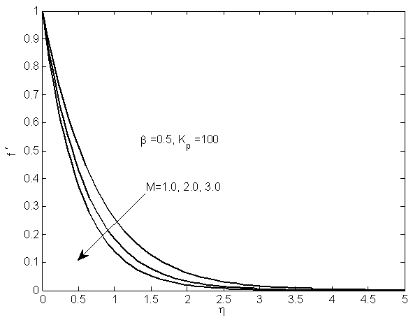
The objective of the present study is to analyze the MHD flow on a stretching sheet embedded in a porous medium. The effects of magnetic field and permeability of the medium on the flow field are to be analyzed. We have considered flow of a conducting viscous fluid through porous media using Darcy model subject to a variable magnetic field. The non-linear equation of the flow field has been solved by Differential transformation empowered by Pade approximants and Runge-Kutta method with shooting technique. The results of both the methods have been compared to establish the consistency of the methods used and accuracy of the result so obtained. It is found that results obtained from both the methods do agree to a certain degree of accuracy. It is also remarked that magnetic field and permeability of the medium contribute to thinning of the boundary layer. Moreover, permeability parameter reduces the skin friction. The relative error of the two methods in computing skin friction ranges from 0.058 to 0.009(Table-2). The error decreases either for higher value of magnetic field or the power index (β). Further as regard to thinning of boundary layer, an increase in magnetic parameter from  to
to  , the boundary layer thickness reduces from 0.1 to 0.06 at η=1.5(Fig. 1).
Keywords: MHD flow, Stretching sheet, DTM Pade, Runge-Kutta, Porous media
Cite this paper: S. Baag, M. R. Acharya, G. C. Dash, MHD Flow Analysis Using DTM-Pade’ and Numerical Methods, American Journal of Fluid Dynamics, Vol. 4 No. 1, 2014, pp. 6-15. doi: 10.5923/j.ajfd.20140401.02.
Article Outline
1. Introduction
- Nonlinear phenomena have important effects on applied Mathematics, Physics, and issues related to Engineering. The variation of each parameter depends on different factors. The importance of obtaining the exact or approximate solutions of nonlinear partial differential equations (NLPDEs) in Physics and Mathematics is the most formidable problem that needs various methods for exact or approximate solutions. Most of nonlinear equations do not have a precise analytic solution; so numerical methods have largely been used to handle these equations. There are also some analytic techniques for nonlinear equations. Some of the classic analytic methods are Lyapunov’s artificial small parameter method [1], perturbation techniques [2-4], and δ-expansion method [5], Adomian decomposition method (ADM) [6, 7], Homotopy perturbation method (HPM), homotopy analysis method (HAM), the DTM, and variational iteration method (VIM) [8, 9].Magnetohydrodynamics (MHD) is the study of the interaction of conducting fluids with electromagnetic phenomena. The flow of an electrically conducting fluid in the presence of a magnetic field is of importance in various areas of technology and engineering such as MHD power generation, MHD flow meters, and MHD pumps [10-12]. Flow through porous media plays an important role in many areas of engineering and industrial interests. In particular flow on a stretching sheet finds wide application in polymer industries. Recently Peker et al [13] and Mohammadreja et al [14] have studied the flow of a conducting viscous fluid over a stretching sheet with a constant rate of stretching and the flow is subjected to variable magnetic field. They have not considered the presence of porous media in their study. In the present study we have considered a stretching sheet embedded in a porous medium with uniform matrix and subjected to a magnetic field strength proportional to
 and non linear stretching
 . Many researchers have considered the strength of magnetic field as constant.The objective of the present study is two-fold. Firstly, to generalize the work of Mohammadreja et al [14]. They have considered the variable magnetic field and they have also applied two methods such as DTM Pade and Runge-Kutta method. In the present study we have added one more forcing force by allowing the flow through porous media and in the presence of a variable magnetic field. Secondly, applying DTM-Pade and Runge-Kutta methods to solve the non-linear equations in an unbounded flow domain and to compare the results of both the methods.
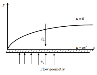
2. Mathematical Formulation
- Consider a steady two dimensional MHD boundary layer flow of a viscous incompressible electrically conducting fluid over a thin flat stretching plate embedded in a porous medium which is placed in the direction of flow. Let the origin of the co-ordinate be at leading edge of the plate, the
 axis be the direction of the uniform stream and the
  axis normal to the plate. A transverse magnetic field of strength
  has been applied perpendicular to the plate. The Prandtl boundary layer- Darcian flow equations subject to above consideration are
  | (1) |
 | (2) |
 and
and  are the velocity components in x and y directions respectively. The symbols
  are the kinematic viscosity, density and electrical conductivity of the fluid. In equation (2), the external electric field and the polarization effects are neglected and the variable magnetic field is given by
 | (3) |
 is the variable porosity given by
  The boundary conditions are given by
  | (4) |
 is the stretching rate.The equation of continuity is satisfied if we choose a stream function
  such that
  Introducing the similarity transformation
 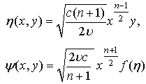 | (5) |
 | (6) |
 | (7) |
 is the magnetic parameter,
  is the permeability parameter and
  is the power index.
 3. Differential Transformation Method
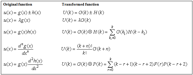
- Differential transformation method is a numerical method based on Taylor expansion. This method tries to find the coefficients of series expansion of unknown function by using the initial data on the problem. The concept of differential transformation method was first proposed by Zhou [15]. It was applied to electric circuit analysis problems. After words, it was applied to several systems and differential equations such as initial value problems [16], difference equations [17], integro-differential equations [18], partial differential equations [19], system of ordinary differential equations [20].
4. DTM-Pade Simulation
- DTM-Padé simulation combines the differential transform method (DTM) and the mathematical theory of Padé approximants to produce a very stable, convergent and adaptable methodology for nonlinear two-point boundary value problems. DTM was originally pioneered in electrical engineering theory by Zhou [15]. It offers analytical solution in the form of a polynomial and can be applied to nonlinear differential equations without requiring linearization and discretization. DTM deviates from the traditional higher order Taylor series method, the latter requiring symbolic computation as the higher order Taylor series needs the computation of higher derivatives and thereby causing greater computational expense for large orders. However, the DTM obtains a polynomial series solution by means of an iterative procedure. DTM is an alternative procedure for obtaining analytic Taylor series solution of the differential equations. With this method, it is possible to obtain highly accurate results or exact solutions for differential equations. Here we provide a summary of the fundamentals of DTM analysis. Consider a function
 which is analytic in a domain T and let
  represent any point in the domain T. The function
  is then represented by a power series whose centre is located at
  . The differential transform of the kth derivative of a function
  is given by:
  | (8) |
 | (9) |
 | (10) |
 | (11) |
 is negligibly small. Usually, the value of m is decided by convergence of the series coefficients. We have documented operations for differential transformed functions about the point
  in Table-1 and we assume that
 in the following sections.
|
5. Pade Approximant
- The polynomials are used to approximate truncated power series. Further, the singularities of polynomials cannot be seen obviously in a finite plane. Since the radius of convergence of the power series may not be large enough to contain the two boundaries, it is not always useful to use the power series. Pade approximants are applied to manipulate the obtained series for numerical approximations to overcome this difficulty. Pade approximant is the best approximation for a polynomial approximation of a function into rational functions of polynomials of given order.Some techniques exist to accelerate the convergence of a given series. Among them the so-called Pade approximant is widely applied (Baker and Morris, [21]). Suppose that a function
 is represented by a power series,
 | (12) |
 is reserved for the given set of coefficients and
  is the associated function.
  Pade approximant is a rational fraction,
 | (13) |
 ought to fit the power series equation (9) through the orders
 . In the notation of formal power series
  | (14) |
 | (15) |
 we get,
 | (16) |
 we define
  for consistency. Since
  equation (13) become a set of M linear equations for M unknown denominator coefficients.
 | (17) |
 may be found. The numerator coefficients
  follow immediately from equation (12) by equating the coefficients of
  such as,
 | (18) |
 .
.6. Application
- In order to solve equation (6), we consider the following boundary conditions:
 | (19) |
 is to be determined.Taking differential transform of equation (6) by using the related definitions given in Table-1, we obtain:
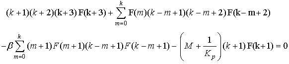 | (20) |
 | (21) |
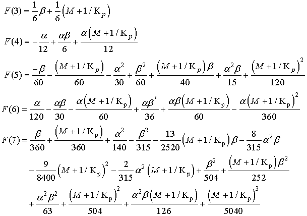 | (22) |
 . The closed form of the solution is
 | (23) |
 =3.0,
=3.0,  =100,
=100,  =0.5)
=0.5) | (24) |
 | (25) |
 α = -0.9748Similarly the other values of α have been determined and are enlisted in the table below.
|
|
7. Results and Discussion
- The effects of various parameters such as magnetic parameter
 permeability parameter
  and the power index (β) as well as the consistency of the methods are discussed in the following lines.Fig.1(a) presents the graphical representation of DTM-Pade method and fig.1 (b) presents the graphical representation of numerical result due to Runge-Kutta method. Both the figures show that the velocity decreases asymptotically with the progress of the flow to reach at the ambient state and the velocity further decreases with the increase of the value of magnetic parameters. The resistive force due to magnetic field is significant in the layers, a little far away from the plate in the absence of porous medium for a fixed value of β. When magnetic parameter increases from
  =1 to
=1 to  =3, the ambient state reaches at about
  (Fig.1a) in DTM Pade method but in case of Runge-Kutta method the ambient state reaches at about
  (Fig.1b). Further, it is seen that presence of porous medium leads to a decrease from the velocity. The effect of magnetic field remains same but the attainment of ambient state becomes faster.Fig.2 (a) and (b) shows the velocity distribution for various values of β =0.5, 1.0, 5.0 representing the integer and fractional values of
 . The value of β=1 correspond to
  i.e. linear variation of velocity and
  , constant magnetic field where as
  and
and  correspond to n=1/3 and -5/3 respectively. This contributes to non linear variation of plate velocity as well as magnetic field strength. The negative power of
 reduces the velocity at all points in comparison with n=1/3
 . On careful analysis from the above observation it is remarked that variation of plate velocity contributes more than the magnetic field strength to increase the fluid velocity in the flow domain.Fig. 3 (a) and (b) represents the velocity distribution due to the presence of porous medium. It is found that velocity decreases at all points of the flow domain. The quantitative values of velocity distribution for porous medium measured at η = 1.5 for both the figures 3(a) and 3(b) reveals that for
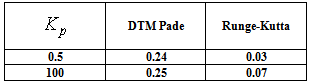
  = 0.5, the convergence is faster by 12.5% due to shooting technique and for non-porous medium it is 28% (Table-3). The result of numerical method indicates the sharp decrease in the profile (fig.3(b)). This shows that the self corrective procedure of shooting technique accelerates the convergence faster than the convergence affected by Pade approximant in DTM. In table-2 and table-3 the error analysis and comparison has been presented.Table-2 shows the values of skin friction obtained by Runge-Kutta and DTM Pade method. It is seen that magnitude of skin friction increases due to presence of porous medium and magnetic field but the power index of magnetic field affects the skin frictions adversely. Results of DTM-Pade and Runge-Kutta method agree to a certain degree of accuracy. The numerical values in both the methods are found to be negative but the accuracy is up to the first place of decimal. The relative error computed ranges from 0.005 to 0.057(Table-2).
 | Figure 1(a). Velocity in y-direction for β=0.5 and Kp=100 |
 | Figure 1(b). Velocity in y-direction for β=0.5, Kp=100 |
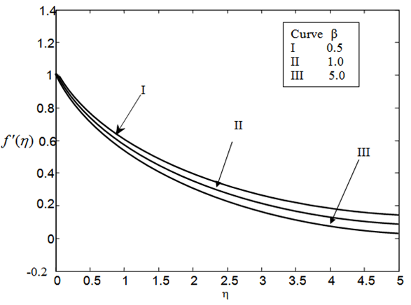 | Figure 2(a). Velocity in y-direction for M=2.0 and Kp=100 |
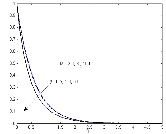 | Figure 2(b). Velocity in y-direction for M=2.0, Kp=100 |
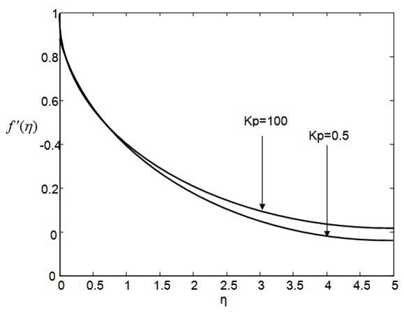 | Figure 3(a). Velocity in y-direction for M=3, β=0.5 |
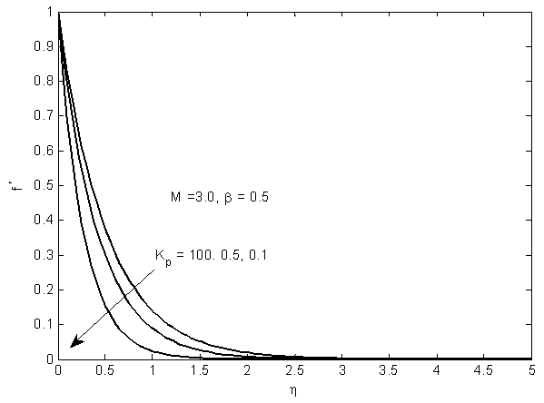 | Figure 3(b). Velocity in y-direction for M=3, β=0.5 |
8. Conclusions
- From the Pade approximant mentioned above it is evident that
 has been approximated by a rational fraction (13) and its approximation given in equation(14).The inclusion of more number of terms will increase the accuracy vis-à-vis increase the order of the diagonal matrix whose inversion is warranted to solve the system of equation. In the present study to avoid the complexity of calculation we have restricted
  to include the term
 that corresponds to [2/2] diagonal Pade. Therefore, it is suggested that if terms of higher powers of
  are considered that will lead to higher order diagonal Pade and consequently better approximation and hence higher accuracy.Due to resistive force of electromagnetic origin i.e. Lorentz force, the velocity decreases. Moreover, the power index as well as permeability of the medium reduces the velocity at all points. The shearing stress over the plate is increased due to permeability of the medium and the magnetic field but reverse effect is observed due to power index of magnetic field.