1. Introduction

Similar solutions to a boundary layer flow are important with respect to the mathematical character of the solutions. In particular the phenomenon of similarity constitutes a considerable mathematical simplification of the problem of solving a system of partial differential equations that arise in boundary layer flows. A goal of this simplification however looks for the type of potential flows for which similar solutions exist.

When the question of similarity solutions of the 2-D steady boundary layer equations arise, there appears two classes of solutions which are characterized completely by the potential flow velocity one of which is where are constants. Falkner and Skan[2] derived this potential flow velocity as a condition for the similarity solutions to exist. Two special cases of the Falkner and Skan similarity solutions are (i) that leads to the famous Blasius[3] solution and (ii) that leads to the Hiemenz[4] stagnation point flow. The other case of the potential flow velocity is are constants) which may be considered as a limiting case of the first case when and which is less explored.

The similarity solutions to the unsteady 2-D boundary

layer equations compared to the steady case mentioned above is much complex due to the fact that the three variables need to be reduced to a single variable, say, Perhaps Rayleigh[5] was the pioneer in this respect. However H. Schuh[6] and Th. Geis[7] have indicated the class of similarity solutions for which a reduction to a single variable is possible such as with is the potential flow velocity and is the scale factor of the ordinate. Potential flow velocity in such cases were taken to be of the form Similarity solutions for the potential flow velocity of the form and b are constants, were analyzed by Yang[8]. In recent time Ma and Hui[1] discussed briefly the three types of similarity solutions of the 2-D unsteady boundary layer equations starting with that of Rayleigh and analyzed those solutions using classical Lie Algebra. Their solutions were, however, limited to the case of taking density and kinematic viscosity Semi-similar solutions of the unsteady boundary layer flows including separation was developed by Williams and Johnson[9] using a simplified scheme. Burde[10] constructed several new explicit solutions of unsteady boundary layer flows some of which appear to be undetected by other similarity reduction method. Following Ma and Hui, Ludlow et al.[11] made a rigorous approach by using one parameter Lie Group to obtain some new similarity solutions of the same boundary layer equations.

An approximate integral method analogous to the Karman-Pohlhausen procedure was introduced by Bianchini et al.[12] to calculate the characteristics of the unsteady 2-D boundary layer flows, but taking the potential flow velocity simply as a function of time Later, this method was modified by Sattar[13] taking the potential flow velocity as a function of where a time dependent length scale was introduced. The first introduction of this length scale to obtain local similarity solution in time of a one-dimensional unsteady heat and mass transfer flow was, to the best of the knowledge of the author, made by Sattar and Hossain[14]. With the aid of this similarity concept, many papers were published by the author and his co-workers some of which are Sattar[15,16], Alam and Sattar[17], Sattar and Maleque[18] and Rahman and Sattar[19]. Seddeek & Aboeldahab[20] and recently Chamkha et al.[21] applied the same time-dependent similarity parameter technique for the solutions of unsteady one-dimensional MHD free convection boundary layer problems.

The objective in this article is to find a similarity reduction of the 2-D unsteady hydrodynamic boundary layer partial differential equations to a single ordinary differential equation, namely a local similarity equation, with a goal to derive the similarity conditions for the potential flow velocity distribution. Unlike the methods adopted so far in solving 2-D unsteady boundary layer equations, a further goal of the article is to extend the idea of introducing the time dependent length scale to obtain the local similarity equation.

2. Mathematical Formulation

Let us consider the unsteady two-dimensional hydrodynamic boundary layer equations which are

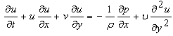(1)

(2)

The boundary conditions corresponding to the above equations are

(3)

where are the velocity components along axis which is the direction of the flow along the boundary and perpendicular to the boundary respectively, is the time, is the kinematic coefficient of viscosity and is the potential flow velocity.

In order to address the question of similarity of the equations (1) and (2), dimensionless quantities need to be introduced. Thus all lengths are referred to a time dependent length scale in line with the work of Sattar & Hossain [14]. Since the -coordinate is mainly related to the boundary layer growth, it is referred to a dimensionless scale factor

Therefore, the following dimensionless lengths are introduced:

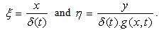(4)

Using (4) a dimensionless stream function is defined as

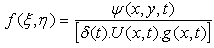(5)

where is the stream function of the boundary layer flow that satisfies the continuity equation (2).

Consequently the velocity components become

(6)

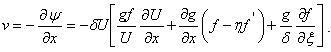(7)

Now from (6)

(8)

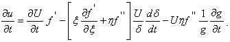
By introducing the dimensionless variables from (4) and (5) along with the equations (6) to (8) into equation (1), the following equation for is now obtained as

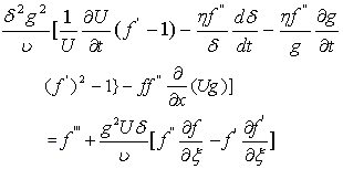(9)

The boundary conditions (3) subject to equations (4) and (5) now reduce to

(10)

In equations (6) - (10), denotes differentiation with respect to

It is, however, seen directly from equation (9) that the velocity profiles are similar when the stream function depends only on the variable defined in (4) with the dependence of being cancelled. This would thus reduce the partial differential equations (1) and (2) to an ordinary differential equation for This reduction would thus lead to the derivation of the expression for the potential flow velocity for which local similar solutions are to exist. Thus under the above assumption equation (9) reduces to

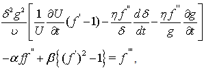(11)

where the coefficients are the contractions for the functions defined as

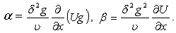(12)

Further we assume that functions are separable and thus and become exactly functions of and hence both can be considered to be proportional to

The above assumptions and the proportionality to have been made to render the equation (11) to a similarity form.

It is thus assumed that

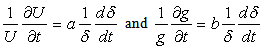(13)

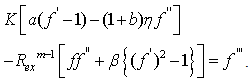
where are the proportionality constants.

Hence equation (11) becomes

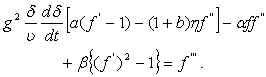(14)

Now the similarity of the equation (14) requires that both must be independent of that is, they must be constants. This condition of consistency, combined with equation (12) will furnish two equations from which the potential flow velocity and the scale factor for the ordinate can be derived and hence the length scale can be evaluated.

Now for the purposes mentioned above, the procedure due to Falkner and Skan[2] is adopted here and thus the following expression is obtained

If now integrating the above expression with respect to one obtains

(15)

Again from (12) one can have

(16)

Integrating (16) with respect to it is obtained that

where is an integrating constant but a function of time

Thus follows

(17)

Now from (15) one has

(18)

Introducing (18) in (17) one obtains

which finally yields

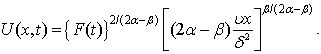(19)

Expressions (18) and (19) respectively yield the scale factor for the ordinate and the velocity distribution of the potential flow. The case has, however, been excluded. Since the above results are independent of any common factor of as long as it is possible to put without loss of generality.

It is, thus convenient to introduce a new constant to replace by taking so

(20)

Hence with the velocity distribution of the potential flow and the scale factor for the ordinate become respectively

(21)

(22)

Now to have a specific functional representation of two choices of the function are made:

(23)

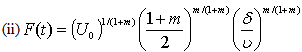(24)

where is a reference velocity.

With the use of (23), from (21) the potential flow velocity turn out to be

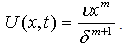(25)

Again with the use of (24), from (21) the potential flow velocity further becomes

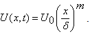(26)

The goal of the present work has thus been achieved which can be viewed from (25) and (26).

One can thus conclude that the locally similar solutions of the unsteady boundary layer equations are obtainable when the potential flow velocity is inversely proportional to a power of and directly proportional to a power of measured along the wall from the stagnation point. The above two forms of so obtained refers to the wedge flow where is the wedge angle. At this stage, the similarity of the equation (14) still remains unresolved because of the term

The above term is now explored by introducing from (22) and from (25).

It thus appears that

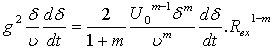(27)

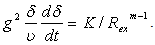
where is the local Reynolds number.

Now the similarity (local) of the equation (14) requires that the term 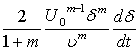in (27) must be a constant. Hence let

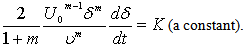(28)

It is now important to look for the time dependency of the length scale which is obtained by integrating equation (28) as

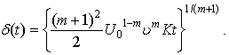(29)

Thus using (28), from (27) we obtain

(30)

Now with the aid of (30), the equation (14) can be written as (with

Without loss of generality it is further assumed that 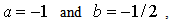so that the above equation becomes

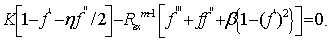(31)

A local similarity equation in the form of an ordinary differential equation of the partial differential equations (1) and (2) is thus obtained, the existence of the solutions of which depends on the condition (25) or (26).

Equation (31) can thus be considered to be a general form of similarity for the 2-D unsteady hydrodynamic boundary layer problem from which the similarity equation for the steady case can be easily extracted.

3. Steady Case

When the flow is steady, is no longer a function of time rather can be considered as a characteristic length such as Thus from (28), we can take

Thus the parameter in (28) in this case becomes identically zero. Hence putting equation (31) reduces to

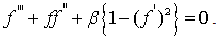(32)

Equation (32) is a recovery of the Falkner and Skan equation whose solution was obtained in details by Hartree[22] for both accelerated and decelerated flows. On the other hand many fold solutions of the equation (32) was obtained by Stewartson[23].

4. Reduction of Eq. (31) to the Case of a Flat Plate

In order to justify the general form of the equation (31) and the derivation of the potential flow velocity represented in (25), let us consider the unsteady 2-D boundary layer flow along a flat plate where so that the potential flow velocity becomes

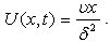(33)

Thus taking the similarity equation (31) turns out to be

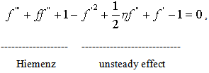(34)

where

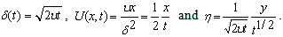(35)

The first part of the equation (34) is the Hiemenz[4] steady stagnation-point flow solution and the 2^nd part is due to the unsteady effect. Equation (34) and the corresponding results (35) thus perfectly agrees with those obtained by Ma and Hui .

The length scale for the ordinate similar to one seen in (35) was initially used by Stokes[24] for an unsteady parallel flow but form of the length scale was initially developed by Sattar and Hossain[14] in case of a solution of an unsteady one-dimensional boundary layer problem. The characteristic length scale defined particularly in (35) physically relates to the boundary layer thickness which can be viewed in Schlichting[25].

5. Results and Discussion

Explicit solutions to steady or unsteady boundary layer equations are important both from theoretical and practical points of view. Such solutions are, however, related to the reduction of the boundary layer equations to a similarity form and to the conditions for the existence of the relevant similarity solutions. In case of the steady boundary layer equations it was earlier established that the similar solutions would exist if the velocity distribution of the potential flow is proportional to a power of the length of arc, measured along the wall from the stagnation point (Schlichting[25]).

In this work the author has thus explored the possibility of obtaining a very simple but general form of a local similarity equation of the 2-D unsteady Prandtl boundary layer equations vis-à-vis the condition for the existence of similar solutions of this equation. This principle has thus led to the derivation of the equation (31) and the condition (25) or (26) for the potential flow velocity distribution. The validity of the equation (31) can however be ascertained by the equation (34) which is a special case of equation (31) and which was earlier established by Ma and Hui[1].

Although the prime goal of the work was to obtain similarity conditions for the existence of unsteady solutions, the equation (31) has been solved numerically in a comprehensive manner by using the efficient computer algebra software Maple-13 (Aziz[26]). The results of this numerical computation are displayed in Figures 1 and 2 in the form of velocity profiles to show the solution trends.

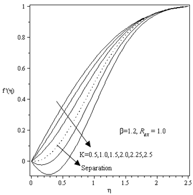Figure 1. Velocity profiles for different values of the unsteadiness parameter

Figure 2. Velocity profiles for different values of

In Figure 1, velocity profiles for different values of the unsteadiness parameter are shown for fixed values of 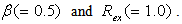It appears from this figure that strong unsteadiness(larger values of ) trigger separation which indicates that back flow occurs close to the surface of the wall. This is due to the fact that strong unsteadiness intensifies the kinematic viscosity of the fluid which causes the decrease of its ambient value and thus results in back flow.

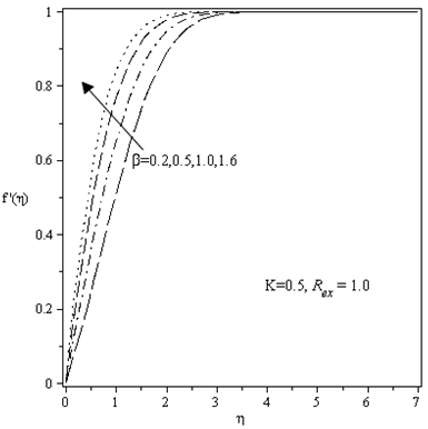
n Figure 2, velocity profiles for different values of at are displayed. Velocity is found to increase with the increase with the increase of which confirms that the velocity profiles for unsteady case follow the same trend of those for the steady case(Schlichting and Garsten[27].

As a comparison of the results displayed in Figures 1 and 2, Figures 3 and 4 respectively are reproduced from Sattar[28] who obtained local similarity solutions of the 2-D unsteady hydrodynamic boundary layer equations of a flow past a wedge. It appears that presents results agree well with those of Sattar.

Figure 3. Velocity profile for different values of K and for β =1.0, Rex = 2.0

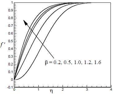Figure 4. Velocity profile for different values of β and for K =0.3, Rex = 2.0

The prime goal of the work was to derive a similarity condition for the potential flow velocity distribution for the existence of the solutions of the 2-D unsteady boundary layer equations and accordingly the condition (25) has been derived which to the best of my knowledge is a new finding. However, for a steady case such a condition is (Schlichting[25]) which corresponds to the condition (25) or (26). Taking the potential flow velocity becomes which is related to flat plate boundary layer (see section 4). Sattar and Ferdows[29] made a similar approach for the similarity solutions of an unsteady free-forced convective 2-D boundary layer flow along a flat plate. Inspired by the work of the author[28], by taking the general form of the of the potential flow velocity, Rahman et al.[30,31,32] obtained solutions to the unsteady 2-D boundary layer problems with heat and mass transfer under various flow conditions. Using the same general form of the potential flow, very recently Muhaiman et al.[33] obtained the effects of thermophoresis particle deposition and chemical reaction on an unsteady MHD two dimensional boundary layer problem.

It is thus apparent from the above works[28,29,30, 31,32,33] that the use of the above potential flow velocity distributions to obtain exact similarity solutions of various unsteady 2-D boundary layer boundary layer problems can make fruitful contributions in computational fluid dynamics research.

6. Concluding Remarks

In this work a comprehensive account of the similarity derivation of the two-dimensional unsteady Prandtl boundary layer equations has been presented. A new class of similarity transformation based on a time dependent length scale has been introduced to obtain a local similarity equation which can be considered to be of general form in contrast to other forms obtained in previous studies. The main findings of the study are now summarized below:

(a) Local similarity solutions of the 2-D unsteady boundary layer equations will exist when the potential flow velocity is proportional to a power of the length scale and directly proportional to a power of the length measured along the boundary in the flow direction from the stagnation point.

(b) The derived similarity equations con be considered as general because both steady and unsteady solutions can be obtained separately.

(c) The similarity equation for the steady case is a recovery of the Falkner and Skan equation.

(d) For a particular case of a flat plate present derivations exactly agree with those of Ma and Hui[1}.

(e) Strong unsteadiness(higher values of ) trigger separation resulting to the back flow.

(f) As in the case of steady flow increase in leads to the increase in the velocity distribution

(h) From the point of fluid dynamics research, particularly in case of unsteady boundary layer problems it can be concluded that the researchers can rely on the general form of the local similarity equation (31) and the corresponding condition for the potential flow velocity derived in (25) or (26).