1. Introduction

The study of aerodynamics will continue to be central to the development of ground vehicle such as cars, trains, and other human powered vehicles. This is driven by the need for improved efficiency in terms of reduced harmful emissions, reduced fuel consumption, increased range and alleviating stability and safety problems. The focus of this paper is on application of numerical aerodynamics to predict forces on a high speed train running in a crosswind.

Time-domain approaches are powerful tools for calculating unsteady aerodynamic forces and moments on ground vehicles running in a turbulent flow. Because high speed trains are constructed with light weight materials to give them higher accelerations and to minimise the power needed to overcome frictional and gravity forces[1], they are susceptible to the risk of overturning, particularly at locations with high crosswinds, such as embankments and open bridges due to local speeding effects. There are also a number of other potential effects – for example turbulent crosswinds can cause dewirement problems with large scale pantograph and contact wire displacements[2]. It is thus important for train designers and operators to ensure that aerodynamic loadings on trains do not infringe their safety limits. Therefore, accurate prediction of unsteady loads on high speed trains in crosswinds is required.

The Quasi-Steady (QS) approach for aerodynamic force calculation is widely used in predicting the response of structures to turbulent wind. The popular use of the QS theory is due to its simplicity and ease of use[3]. Using QS theory, the unsteady aerodynamic force F(t) on a high speed train moving at velocity V in a crosswind is given as

(1)

where is the mean force, is the fluctuating force component, ρ is the air density, is a reference area, is the mean (time-averaged) force coefficient, U is the mean crosswind speed and is the fluctuating velocity. The quasi-steady force as defined in (1) incorporates second order terms associated with the turbulent velocity , i.e. a non-linear quasi-steady approximation. The form of the QS approach as in (1) is a variation of the linearised QS theory where second order effects are not accounted for, i.e.

(2)

It was shown in[5] that the nonlinear quasi-steady approach produced time series of wind-induced shear force coefficients that were more accurate compared with measured values, in contrast to results obtained using the linearised quasi-steady such as in the study of Letchford et al.[5]. From (1) and (2), the unsteady force F(t) follows the history of the instantaneous turbulent velocity , i.e. they are fully correlated. Thus, the QS approach considers the fluctuations due to instantaneous turbulence and neglects the unsteady memory effects of preceding turbulent velocities.

However, unsteady events like flow separation does not have an instantaneous effect but develop its influence on the body surface over a period of time. Tielman[8] discussed how the quasi-steady theory may only be applicable for the prediction of aerodynamic forces in stagnation regions, while failing to predict these forces in separated regions. It was shown previously that ‘building-generated’ turbulence plays an important role in the induced pressure forces, e.g. Cook[6], Letchford et al.[5] and Simiu et al.[7]. The implication is that not all fluctuations of upstream flow are transmitted to the building. For a train passing through a crosswind and for which the forces are simulated at given points along a track, the effect of a turbulent crosswind at one point would still exist at neighbouring points. Preceding turbulence becomes more important if the simulation points are more condensed due to increased spatial correlation.

Another drawback of the QS model is its overestimation of the unsteady forces. In a study on long span bridges[3] it was found that the QS theory was only valid at very high-reduced velocities for which the frequency-dependent fluid memory effects are insignificant. In another study on the effects of crosswinds on a vehicle passing through the wake of a bridge tower, Charuvisit et al.[9] pointed out that the conventional quasi-steady method gives larger overestimation for many cases. Letchford et al.[5] applied the quasi-steady theory approach to compute pressure distributions on a building and found deviations away from the theoretical prediction in separated flow regions as a result of ignoring the building-generated vortices. Clearly, the more aerodynamic information about the flow behaviour around the vehicle is taken into account, the more accurate is the prediction of unsteady forces. Despite these limitations, the QS approach remains a simple method for quick calculations of the effects of winds on vehicles and other structures.

An alternative approach for calculating the unsteady crosswind forces on a vehicle is via the aerodynamic admittance function. This method is not new, dating back to the early works of Sears[10] using thin airfoil theory. Aerodynamic admittance functions, relating the lifting force on a streamlined section to the vertical fluctuating component, were developed through the so-called Sears function[10]. Extending the idea from aeronautics to wind engineering, Davenport[11] introduced admittance functions that relate the wind fluctuation to the wind-induced pressure on structures in the frequency domain. In Davenport’s formulation, the role of the aerodynamic admittance function is to account for the lack of correlation between the velocity fluctuations in the flow region adjacent to the body. However, for a bluff body such as a high speed train, the theory of thin sections is invalid owing to characteristic differences in the flow behaviour between thin and thick sections. For the latter, the aerodynamic behaviour is affected to a large degree by the boundary layer separation, typically involving large-scale strong vortex shedding. For a train with multiple car units, parts of the vehicle will be subjected to a strong wake generated from the leading car. A new fluctuating force component, often referred to as self-buffeting, is induced as a result of signature turbulence (e.g.[12]). In this case, the aerodynamic admittance function should take full account of the unsteady effects associated with signature turbulence. This has led to new definitions of the aerodynamic admittance functions using both computational and experimental tools (e.g.[12]) in an attempt to produce accurate formulations. Computationally, various approaches have been proposed with varying degrees of complexity in their application; see for instance the works of Scanlan[13] and Hatanaka et al.[14]. Such analysis is, however, beyond the scope of this study.

This paper is concerned with numerical estimation of aerodynamic admittance function based on data from experiments on train models. Aerodynamic admittance functions can be defined, in the frequency domain, to relate the spectrum of the inflow velocity fluctuations to the that of the measured forces experienced by a model train in a wind tunnel[15] or in a full scale experiment[16]. As noted by Baker[17], due to difficulty in computing amplitude and phase parameters of an admittance function in the frequency domain, doing the analysis in the time-domain is more convenient. The equivalent expression of aerodynamic admittance function in the time-domain is called the aerodynamic Weighting Function (WF). Using the WF, Baker[17] showed that the fluctuating force may be obtained through a simple convolution of the turbulent wind and an experimentally determined WF. The use of this method has been highlighted in many studies e.g.[18]. Using the definition of the relative wind speed as

(3)

The unsteady aerodynamic force using the WF is[17]

(4)

where = , is a time lag, and h_F () is the aerodynamic weighting function of the force. Compared with equations (1) and (2), the main difference in (4) is the introduction of an integral expression for the fluctuating force component that involves h_F () and a time lag. It can be seen from (4) that the unsteady force histories on a train due to crosswind can be determined from the velocity time histories if the appropriate force coefficients and weighting functions are known. The WF allows the total force F(t) to be related not only to the instantaneous turbulence but also to preceding turbulent velocities within a time lag. Unsteady crosswind forces depend on many parameters like the mean wind speed, the vehicle speed and the turbulent wind. For the WF approach, the aerodynamic weighting function and the time lag are also important.

In this paper, the QS and WF approaches are compared when computing the unsteady side force on a high speed train at discrete simulation points in the presence of a turbulent crosswind. The comparisons are based on the variation of three main parameters: the mean crosswind U, the train speed V, and the simulation distance between the simulation points. The aims are twofold: 1) to show which approach is more accurate and 2) to investigate the range of applicability. In order to increase the accuracy of simulation for the unsteady crosswind force on a high speed train, a simple, practical, and accurate representation of the wind load is the primary motivation of this research work.

2. Methodology

2.1. The Simulated Problem

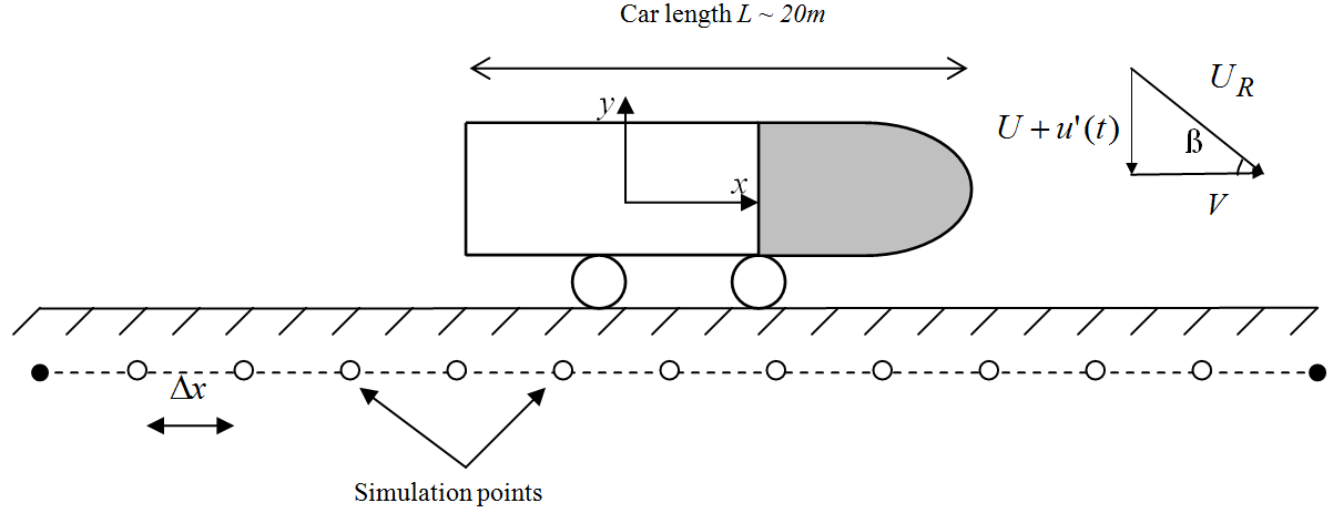Figure 1. Coordinate system, the train/wind velocities, and track definition

In order to compare the two methods, the side force is computed on the leading car of a UK high speed train, the Class 365 Electrical Multiple Unit (EMU), running along a 1 km straight track subjected to an unsteady crosswind normal to the train’s direction of motion. The side force is estimated at discrete points along the track, the number of which is controlled by the separation distance . Figure 1 illustrates the simulated problem where the leading car of length L moving at velocity V is subjected to a crosswind .

The resultant relative velocity that impinges on the train is , is the relative wind angle or yaw angle, i.e. = tan⁻¹ (V/ (t)).

2.2. Outline of the Numerical Method

The numerical procedure to compute the side force consists of the following:

(i) Generation of a turbulent crosswind velocity time history via a spectral approach

(ii) Experimental determination of mean force coefficient as a function of relative wind angle

(iii) Calculation of the aerodynamic weighting function of the train

(iv) Convolution of the weighting function with the fluctuating velocity gives the crosswind force on the train; this is then added to the mean force to get the total unsteady force

(v) For a range of parameters, the two approaches are compared e.g. in terms of mean force value, standard deviation, ratio of standard deviation to mean, and force spectra.

Regarding point (v), since the magnitude of unsteady force is a function of relative velocity then it is natural to be interested in studying how the force varies with mean wind speed, train speed, and gust distribution. But one essential fact about the force along the track is that the larger the number of simulation points along the track, the more information it is possible to gather about the force history. When the distance between the simulation points along the track is reduced, the fluctuating velocities become spatially more correlated, so that the unsteady force will exhibit increased sensitivity to the spatial distribution of velocity. This is why it is convenient to compare the two approaches with varying distances . The distance is a key parameter for comparison because the effect of the WF integral in (4) becomes more significant with decreasing this distance as also controls the time lag. In practice, frequencies associated with unsteady flow at certain distances may coincide with the natural frequencies of the vehicle (e.g. its suspension) and so under certain conditions these could be excited, resulting in potential detriment to the vehicle safety.

2.3. Simulation of Turbulent Crosswind

The crosswind flow past the train is assumed two-dimensional, incompressible, isothermal and turbulent in the whole flow domain. The turbulent fluctuation u’(t) is specified by the longitudinal velocity fluctuations at the simulation points along the track. The spectral approach is used to provide a means of simulating a turbulent crosswind field as a stationary random process[18]. The simplicity of the spectral approach is an advantage of time-domain simulations. The turbulent velocities are predicted at every . Full details of the simulation procedure can be found in[18]. For the crosswind velocity time series simulation, each time history at a given point was generated with a sampling rate of 0.167 seconds with a simulation period of ~ 8533 seconds. All realisations were equally spaced in time. The outcome of the spectral approach is a time series of a multi-point correlated crosswind velocity field. It is sufficient to note that in all cases the time series are appropriately correlated to one another and have coherence properties as described by Davenport’s coherence function[18]

(5)

where is the angular frequency, C_Z is a constant decay factor taken as 10, and is the distance between points and , i.e. = . The mean crosswind speed is measured, conventionally, at height = 3 m above the ground. The turbulent wind also conforms to Kaimal’s empirical wind spectrum[11] as given by

(6)

where is the shear velocity defined as

(7)

The shear velocity depends on the ground roughness z₀ (assumed z₀ = 0.03 m for open country terrain). A sample time-series of crosswind velocity is given in Figure 2(a) for U = 22 m/s. The actual wind as seen by the moving train is the vector addition of the wind time series u_w and the train velocity V. Figure 2 (b) shows fair agreement between the target longitudinal Kaimal’s spectrum[19] and the one simulated via the spectral method.

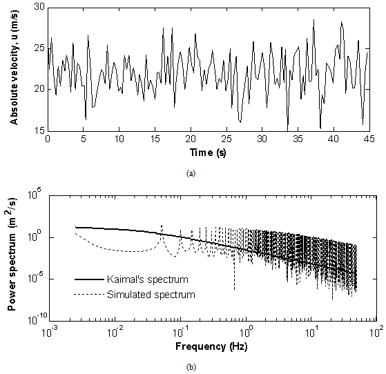Figure 2. Spectral simulation results: (a) crosswind velocity, (b) spectra

2.4. Prediction of Unsteady Aerodynamic Forces

In reality, the behaviour of the wind profile around a moving vehicle is not simple. The resultant velocity field from a moving vehicle and an atmospheric boundary layer profile results in a skewed boundary layer profile as explained by Hucho and Sovran[20]. Due to the nature of wind, one expects the response of the train due to crosswind to have two components: 1) a quasi-static response as a result of the mean velocity and low frequency fluctuations, and 2) a response due to high frequency wind fluctuations that are the source of dynamic excitations. To determine the unsteady forces on a train due to crosswind either through the QS or the WF theory, two pieces of information are required: records of wind speeds, and variation of force coefficient as a function of yaw angle. While the wind history is obtained from the spectral simulation, the force coefficients were obtained from wind tunnel tests of a Class 365 scaled model, according to experimental details in[21]. The force calculation using the WF is as follows. The method builds on the one developed by Baker[17] for a moving vehicle, which requires determination of an aerodynamic admittance function from experimental data. Based on a linearised analysis in the frequency domain, Baker[1] expressed this function in terms of measured quantities as

(8)

where is the aerodynamic admittance function, and n is frequency in Hz. In (8), and are the power spectra of the force being considered and longitudinal wind velocity, respectively. Clearly, the admittance function is frequency-dependent. In the time-domain, the weighting function appearing in the unsteady force equation (4) is the Fourier transform of the transfer function in (8). Thus, if the admittance is known, the weighting function can be found as a function of train geometry, yaw angle, etc. This is not usually the case, however, as wind velocities and forces are not usually measured sufficiently close together in time to enable to be determined[17]. Therefore, the following approach is adopted. From wind tunnel tests, the force admittance functions as defined in (8) are plotted against the yaw angle, as illustrated in Figure 3.

The immediate observation is that all admittance functions drop off at high frequencies, roughly to about a tenth of their value at lower frequencies. The decrease of aerodynamic admittance with increasing frequency is expected because at higher frequencies the smaller turbulent eddies have shorter wavelengths and thus have a more rapid loss of coherence than for the larger eddies[7]. These admittances are then transformed into the time domain to yield equivalent aerodynamic weighting functions. By fitting curves to data in Figure 3, it can be shown that the weighting function for the Class 365 could be written as

(9)

where , L is the vehicle’s length (~ 20 m), and the weighting function time lag appearing in (4). The weighting functions are thus found from the measured admittance functions, thereby enabling calculation of the unsteady force in (4). Now that the weighting functions are computed, the unsteady forces are obtained by adding the averaged and fluctuating parts as defined in (4). The fluctuating part F’(t) in (4) can be computed either in the time domain by expressing the integral as a convolution * (since the system is causal), or in the frequency domain by taking a Fourier transform for F’(t) which changes the integral to a product of the Fourier transforms of and , and then taking an inverse Fourier transform of the result.

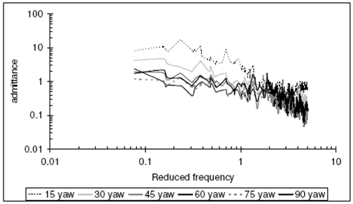Figure 3. Side force admittance function for a 1/30th scale model of the Class 365 EMU[21]

2.5. Discussion of the Aerodynamic Weighting Function

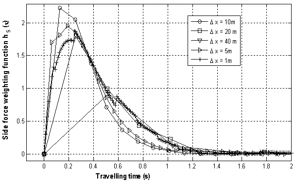Figure 4. Side force weighting function for different separation distances , U = 25 m/s, V = 80 m/s

The weighting function represents the contribution of preceding turbulent crosswind velocities to the current value of unsteady force. There is a higher weighting for points closer to the current simulation point , which then reduces for points far apart, showing the physical effects of spatial correlation. This is in contrast to a moving average filter for which equal weighting is usually applied. In a discrete formulation the side force F_S may be written as

(10)

From (10), it is seen that the effects of the weighting function, and thus the fluctuating force, become more important if the integration time step is very small. The can be reduced making smaller, implying a larger number of simulation points. This is, however, numerically more expensive due to the need to simulate a larger number of turbulent velocities via the spectral approach. Another important characteristic time scale is the time period of the weighting function after which the weighting function is zero. The weighting function may be regarded as a low pass filter which smoothes high frequency, short period fluctuations of periods less or equal than , and diminishes any fluctuations for time periods where the weighting function falls to zero as time increases beyond . The time step in the integration of the weighting function is the same as the time step for force calculations. Hence, the train speed V also affects the size of in addition to since roughly . The mean crosswind speed U is also important since it appears in Kaimal’s spectrum definition. Sample forms of the side force weighting function h_S (t) for different separation distances at constant V and U are shown in Figure 4. For the cases shown, although the weighting function’s characteristic time scale is the same for all separation distances (~ 1.2 s) the filtering effects are more pronounced with smaller distances .

From force definitions, the form of weighting function as seen in Figure 4 will affect the resulting unsteady aerodynamic force. It is noted in passing that the WF approach applied to a high speed model was used successfully by Ding[18] to reconstruct some experimental data.

3. Study Cases

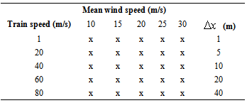
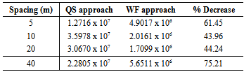
In order to investigate the sensitivity of the two force calculation approaches, a matrix of three parameters of mean wind speed U, train speed V, and separation distance was used in this study as summarised in Table 1. From Table 1, the implication is that that 25 simulation cases are required because the turbulent velocity field depends on both the mean crosswind speed (through Kaimal’s spectrum) and the separation distance (through Davenport’s coherence function), but is independent of train speed. To obtain the unsteady force for the full matrix of these parameters a total of 125 force computations are required. However, only some selected cases will be studies and discussed. The comparison between the two approaches in each case is considered in three ways: standard deviation of the force (and its ratio to the mean force), the force power spectra, and variances.

Table 1. Matrix of Parameters for Unsteady Force Calculations with QS and WF Approaches

3.1. Comparison of Unsteady Force Time Histories

In order to illustrate the effects of the WF on the unsteady force compared with the QS theory, two time histories of side force acting on the Class 365 EMU train are plotted together in Figure 5 (b) in response to the crosswind velocity history (for U = 25 m/s and = 10 m) of Figure 5 (a), illustrating how the WF filters the high frequency content. The force signal due to the WF is also slightly delayed compared with the QS force signal which follows the velocity history exactly. No vehicle suspension effects were included when computing the unsteady forces. From the unsteady force definitions for the QS and WF approaches, the main difference is how the fluctuating part of the force is accounted for. Since the force standard deviation, F_std, is a measure of the spread of data from a mean value it is appropriate to use it as a parameter to distinguish the effects of turbulent fluctuations for each calculation method. With reference to Table 1, for each train speed, five standard deviations are computed corresponding to five mean wind speeds. Each value of F_std is computed from the total force time history as the train travels a 1 km track. Results for side force standard deviation at different mean wind speeds are shown in Figure 6 for a train with V = 80 m/s and = 5 m.

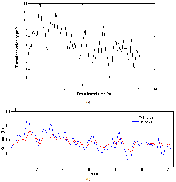Figure 5. (a) simulated turbulent crosswind, (b) Unsteady forces

Several observations can be made by looking at Figure 6. In both approaches the force std increases with increasing mean wind speed due to increased level of fluctuations, in accordance with Kaimal’s spectrum of longitudinal turbulence, see (5). However, when the std of both approaches is compared at the same mean wind and train speed, the std is higher in the QS approach than in the WF method due to the velocity fluctuations in the QS theory being unfiltered as opposed to the WF method in which force fluctuations are filtered via the WF integral. Although not shown, this trend in force std between the two methods was found for all the train speeds. For the specific example illustrated in Figure 6 the std for QS theory is almost twice the std of the WF approach, illustrating the smoothing nature of the WF method.

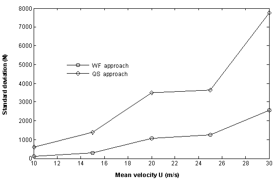Figure 6. Variation of side force standard deviation with mean crosswind speed between the QS and WF approaches

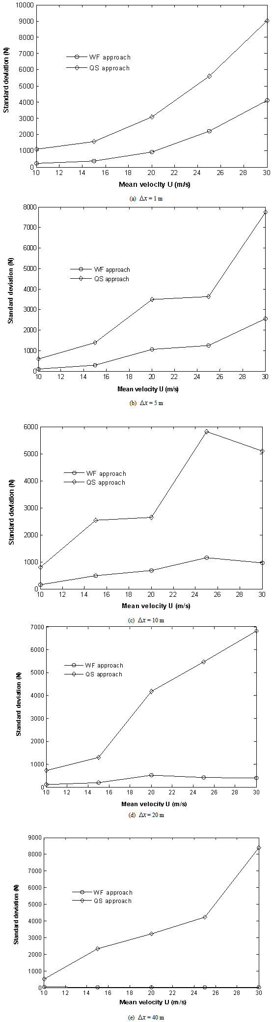Figure 7. Variation in side force std due to WF and QS as is varied from 1 m to 40 m for all mean wind speeds (V = 80 m/s)

If the std of the side force is compared at a constant train speed of V = 80 m/s but different separation distances and for all mean wind speeds the results are plotted in Figure 7. The immediate observation is that when the separation distance decreases the std of the force increases for the WF, presumably due to increased number of turbulent velocities fluctuating off the mean. However, it is lower than the QS approach where it remains quite high for all separation distances. The higher filtering effect of the WF at larger separation distances is clearly visible, particularly at = 40m where the std is negligible. This is caused by a larger force integration time step at larger as shown in the definition of the WF integral of Eq. (4) which causes the WF to become zero rather quickly (the WF completely damps out most fluctuations). Thus, at = 40m the unsteady force is overly-filtered and becomes a constant value.

3.2. Frequency Analysis of Force History

In this section, the unsteady forces due to the WF and QS approaches are compared when the train passes through sinusoidal gusts with single frequencies. In principle, the power spectra of both approaches should reproduce the main frequency of the sinusoidal gust. We consider gust time histories of the form

(11)

where A is the gust amplitude, is the gust radian frequency (= 2πf, f frequency in Hz), and t is the time. Since the train travels at different speeds and the forces are computed at different separation distances, the sampling frequency for the forces will depend on these two parameters. Hence, only specific gust frequencies will be captured by the train without any aliasing for a given train speed and separation distance. For example, when the train speed is 80 m/s and = 10 m, the sampling frequency of the force is 8 Hz. Thus, by the Nyquist theorem only gust frequencies of Hz may be seen by the train. For constant amplitude gust with three different frequencies (1, 2 and 3 Hz) the unsteady forces and corresponding spectra of both approaches are shown in Figure 8.

A sinusoidal crosswind gust is a deterministic model which is fully correlated along the length of the track. As expected, the sinusoidal crosswind excitations lead to sinusoidal side force. It is seen that the power spectra produced by both approaches give the correct spectrum for each gust frequency. This indicates that the current method of force response to sinusoidal gusts produces accurate results. However, despite the mean force being the same, the fluctuating part due to the QS approach is higher than the one due to the WF method.

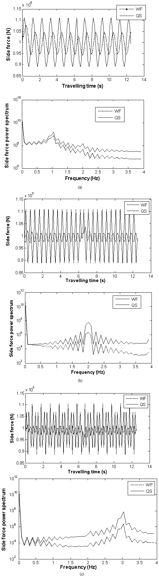Figure 8. Force histories due to sinusoidal gusts and their power spectra: (a) f =1 Hz, (b) f =2 Hz, (c) f =3 Hz

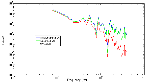Figure 9. Force power spectra comparison between the WF and QS approaches (U = 25 m/s, V = 80 m/s, = 10 m)

The weighting function works in a similar way to a digital filter in which a weighting is applied to a sequence of discrete data points in a time series. Similar to a digital filter, temporal filtering through the WF has an effect on the characteristics of the structure of the force signal such as its power spectrum. It is the purpose of this section to briefly explore the implications of filtering through the WF on some turbulence statistics including variance, and on the power spectra. The fluctuating force component in Eq. (4) may be re-written discretely as

(12)

where is the filtered force at time , h_j is the weighting applied to the fluctuating velocity simulated at time , is the number of time lags over which the WF is applied to the values preceding the current relative velocity . Because of filtering, a loss in the force magnitude and its variance is expected. In order to illustrate the role of filtering due to the weighting function as compared with the QS approach, the power spectra of the side force in both approaches are compared for different spacing between the turbulent velocities. One expects the decrease in the slope of the power spectra at high frequencies to be greater as a result of filtering due to the WF. Figure 9 shows the difference in slope at high frequencies between the QS and WF methods. As seen from Figure 9, the WF power spectrum (plotted on a log-log scale) has a roll-off in the higher frequencies (higher mean slope) compared with the QS spectrum (both linearised and non-linearised forms).

The spectra are not smooth presumably because of turbulent noise as part of the spectral simulation. At low frequencies, whilst the linearised QS and the WF methods have nearly the same power, the non-linearised QS approach has a slightly higher power due to the contribution from second order terms. At higher frequencies, however, the power spectrum from the WF method falls more rapidly compared with both versions of the QS approach which are very similar. This illustrates the effects of the WF which completely dampens out higher frequencies. The contrasting performances of the WF in the time and frequency domains are typical of some filters such as the moving average filter [22] where good performance in the time domain results in poor performance in the frequency domain, and vice versa (e.g. the moving average is excellent as a smoothing filter (time-domain) but can be an exceptionally bad low-pass filter (frequency domain)).

3.3. Variation of Cutt-off Frequency with Separation Distance

This section explores how the cut-off frequency for the weighting function changes with separation distance when the mean wind and train speeds are fixed. For three separation distances of 1 m, 5 m, and 10 m the spectra of side force for both prediction methods are shown in Figure 10 for a mean cross wind of U = 25 m/s and V = 80 m/s.

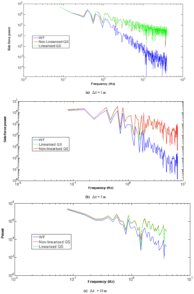Figure 10. Variation of cut-off frequency with separation distance

When the separation distance is smallest at 1m, the behaviour of the power spectrum between the two methods resembles more what is expected: in the lower frequency range, the power spectra collapse on a single line. At higher frequencies, however, the power spectrum due to the WF approach decreases more rapidly compared with the two versions of the QS method. It is evident that sampling the force at smaller separation distances, i.e. at smaller force integration time steps, results in the power spectrum being better defined at a larger frequency range (extended range due to ability to resolve higher frequencies according to Nyquist theory) as well improving the accuracy of the WF at low frequencies (power spectra being the same as expected). From the spectra plotted, the energy starts to fall at the cut-off frequency of about 1 Hz for all sampling distances. Variation of force variance with separation distance

Table 2 shows the decrease in side force variance due to the WF compared with the QS approach for four cases of spacing (for fixed U and V).

Table 2. Decrease in force variance due to filtering by the WF for U = 25 m/s V = 80 m/s

4. Discussion

The separation distance for the multi-point correlated crosswind velocity field is a crucial ingredient in deciding which approach is the most suitable for unsteady force calculation. At larger distances, the WF almost filters out all the turbulent fluctuations, giving a conservative estimate of unsteady aerodynamic effects which are otherwise important for dynamic analysis. This, however, improves as the WF function time lag is decreased, i.e. smaller separation distances, so that the calculation is smoothed over a larger number of preceding turbulent velocities. In a dynamic sense, it implies that unsteady fluid memory effects due to older crosswind velocities on the train are taken into account. On the other hand, the QS approach is likely to overestimate the unsteady aerodynamic force as reported in other studies, leading to unnecessary design contingencies. The improvement in prediction through the WF approach comes at an increased computational time because the velocity field along the track contains a larger number of turbulent velocities that are simulated via the spectral approach. Further work is needed to investigate the sensitivity of the unsteady forces, and thus of the calculation methods, to the full range of simulation parameters.

5. Conclusions

An important conclusion of this paper is that the computation of unsteady force histories with large spatial differences between the simulation points entails loss of correlation between the velocity perturbations and hence the temporal flow development filters out the physical effects of a correlated crosswind field. The solution is to use a condensed sequence of simulation points for turbulent velocity along a track. The reliability of the method of extracting the forces from the turbulent crosswind is examined via two different approaches: the classical quasi-steady theory and the weighting function method. While the QS theory produces increasingly higher force fluctuations as the simulation distance decreases, the WF provides a smoother form of a force signal which removes the short-term high frequency oscillations by applying different weightings to older velocity histories. The ongoing analysis has illustrated the effects of the weighting function on the characteristics of the unsteady side force on a high speed train. Because of its filtering effect, using the WF will be useful in damping out undesirable levels of noise both in numerical as well as physical experiments. Reliability of the WF is, however, strictly limited to using very small time steps.