1. Introduction

Different types of surface facilities are used for phase separation in the oil industry[1-2]. Gravity-based facilities include horizontal three-phase separators consisting of large cylindrical vessels designed to provide a sufficient residence time for gravity-based separation of liquid droplets. The gravity settling approach requires very long cylinders which is not practical and inconsistent with the space restrictions in the oil fields especially offshore. Hence, three-phase separators are equipped with different types of internals to enhance droplet coalescence and optimize their length. A momentum breaker device is implemented at the inlet of the separator to reduce the high inlet velocity of the mixture. At this stage, the liquid phase is separated from the gas forming two distinct layers. Further downstream, perforated plates are used to stabilize the liquid mixture forming two distinct layers of water and oil. These two layers are separated by a weir placed at the end of the separator between two outlets for each liquid phase. The gas phase leaves from its own outlet at the top of the separator.

The design approach of three-phase separators is based on semi-empirical formula obtained from Stokes law[1]. The resulting equation, for the settling velocity based on a chosen cut-off droplet diameter, contains a correction factor which depends on the separator configuration[3]. Although useful guidelines are provided by this approach, crucial information, affecting the separator performance, is not considered. At the inlet of the separator, different flow regimes do occur and a realistic droplet size distribution needs to be considered and tracked throughout the separator compartments to take into account the effects of coalescence and breakup. The internal multiphase flow is assumed to be stable with three distinct gas/oil/water layers separated by sharp interfaces. This is not always the case since previous studies showed that several complex phenomena could take place under different conditions such as liquid re-entrainment[4], recirculation zones within the liquid layers[5], and a dispersion emulsion band between the oil and water layers[6] or foaming[7].

The abovementioned limitations, of the semi-empirical approach, invoke the need of more fundamental and thorough methods based on first principles for a more consistent design of separators and assessment of their performance. Experiments represent a viable alternative or complement as they can replicate real cases under realistic conditions and provide more details using different measurement and visualization techniques. However, experimental techniques are costly and very difficult to apply for sizes approaching real scale and using real fluids. Consequently, only few studies have dealt with such large scales for limited purposes as done by Simmons et al.[8] for the estimation of the Residence Time Distribution (RTD) based on experiments with tracers. On the other hand, studies using laboratory-scale separators do exist in the literature although for specific purposes as well. Waldie and White[9] studied the damping effect of the baffles using electrical conductance level probes. Simmons et al.[10] devoted their study to the RTD measurement using spectrophotometer placed downstream of the liquid outlets. Jaworsky and Daykowski[11] used a transparent separator to test their distributed capacitance sensors. The experimental investigations remain crude with a focus on global parameters. Details of the internal flow field and phase compositions still remain elusive with present day techniques.

Computational fluid dynamics (CFD) represents an alternative tool gaining more confidence within the industrial community due to the development of more robust numerical and physical models and the huge development in terms of computing resources. It is more universal than the semi-empirical models and more flexible than the experimental techniques. Among previous studies we can mention those developing appropriate models to take into account the droplet size distribution in conjunction with coalescence and breakup phenomena[12-14] or to understand the effects of certain parameters on the separator performance and internal flow[15-16]. Industrial investigations which focused on parametric CFD studies for debottlenecking purposes include[17-19].

Due to the complexity of the multiphase flow in horizontal gravity separators, simplifying assumptions were always necessary which limited the accuracy of the CFD approach to an acceptable scale from an industrial point of view and provided useful guidelines for design and troubleshooting of operational problem. The multiphase flow was usually assumed to include only two phases while three-phase simulations were scarce. The Reynolds averaged Navier-Stokes-based (RANS) k-ε turbulence model, the work horse in industrial CFD, was combined with multiphase models due to its robustness, simplicity and reasonable computational cost[20]. Baffles were modelled as porous media. Last but not least, mono-dispersed secondary phases were frequently imposed excluding any possibility for droplet size variation either by coalescence or breakup especially within the Lagrangian framework.

Therefore, only few contributions dealt with the secondary phases as poly-dispersed. Hallanger et al.[21] developed a CFD model based on the two-fluid model approach to simulate the three-phase flow in a 3.15mx13.1m horizontal gravity separator. They neglected the effects of gas flashing, foaming and emulsification, interactions between dispersed phases, droplet breakup and coalescence. They represented the oil dispersed phase by an average diameter equal to 1000 μm and the water phase by 7 groups of sizes with an overall average diameter equal to 250 μm. They found that most of the water droplets, smaller than 150 μm, were entrained by the oil phase while most of those larger than 500 μm were efficiently separated. Song et al.[12] proposed a method to include the drop size distribution in sizing gravity separators through the Sauders-Brown equation. The equation required an appropriate k factor for gas-liquid separation and a realistic retention time, obtained from laboratory or field tests, for liquid-liquid separation. The method was tested on a 4.42mx15.85m separator. They obtained a cut-off diameter equal to 90 μm for the oil and water droplets entrained by the gaseous phase. In addition, 4.5% of water-in-oil would be lost in the oil outlet with droplets smaller than 225 μm and 3500-4000 ppm of oil-in-water would be lost in the water outlet with oil droplets smaller than 60 μm. Grimes et al.[13] developed a Population Balance Model PBM for the separation of emulsions in a batch gravity settler. The model considers the interfacial coalescence, using a film drainage model, and the deformation of the emulsion zone due to the dynamic growth of the resolved dispersed phase. In addition, the accumulated buoyancy force in the dense packed layer and the hydrodynamically hindered sedimentation are also considered. The model developed by Grimes et al.[13] was tested by the same authors[14]. They used data obtained from experiments on gravity-based separation of a heavy crude oil with two different, 10 ppm and 50 ppm, concentrations of de-emulsifier using low-field Nuclear Magnetic Resonance. The tests, focusing on the dispersed water phase, permitted the calibration of the model. The study highlighted the importance of poly-dispersity and its effects on the coalescence rate and the separation rate by sedimentation. The authors noticed that isolated small populations of the smallest droplets would aggregate above the active coalescence and sedimentation zone permanently and might form regions of non-separated components with possible relatively high concentrations (10%) due to the complex physics of collision and coalescence, combined with a simultaneous sedimentation for poly-disperse emulsions. Nevertheless, they mentioned the low performance of the hindered sedimentation rate model, which didn’t account for poly-dispersity satisfactorily, and noticed some discrepancies with increasing residence time.

In addition to the general simplifying assumptions found in the literature, a major limitation is associated with the multiphase models themselves. ANSYS FLUENT includes several multiphase models belonging to both the Lagrangian and Eulerian approaches[22]. The Eulerian approach includes the volume of Fluid (interface tracking model), the mixture, and the Eulerian-Eulerian models. The volume of fluid model is able to predict the interfaces, separating the components, accurately but is limited by the demanding computational resources, for a sufficiently fine mesh. The mixture model includes an additional equation for the prediction of the slip velocity and is limited to mono-dispersed secondary phases. It is worth mentioning that the turbulence models used in conjunction with the two previous models are the same as those used for single phase flows. The Eulerian-Eulerian model solves individual momentum equations for each phase and can be combined with appropriate multiphase turbulence models but still limited by the mono-dispersed secondary phases. In addition to the size distribution limitation, the Eulerian models, being based on inter-penetrating media assumptions, do not consider coalescence or breakup of particles. The Discrete Phase Model (Lagrangian particle Tracking) is a remedy for the limitations related to the size distribution, coalescence, and breakup. However, it requires a background phase to interact with. Thus, an Eulerian model is used to obtain the overall flow structure, which in the case of separators and depending on location inside the domain of integration, is characterized by three background phases for the DPM particles. Nevertheless, the Eulerian multiphase models consider only a single continuous phase throughout the computational domain. This assumption contrasts with the fact that the continuous phase changes inside the separator as we move from one region to another. In this case, the interaction of the DPM particles with the background Eulerian phases is omitted in a relatively important portion of the computational domain. This limitation can be overcome by the Population Balance Model used in an Eulerian framework. The PBM solves a transport equation for the number density function tracking, thus, the droplet size distribution inside the whole computational domain while, at the same time, accounting for the effects of coalescence and breakup. In its present form however, the PBM model is also limited to a single secondary phase. So, the other secondary phase is represented by a mean representative diameter. To the authors knowledge, apart from the work of Grimes et al.[13-14] batch gravity separation of oil/water emulsions, the PBM model was not used to study three-phase separators.

In the present work, the PBM model is used to include the effects of the droplet size distribution on the separator performance and the internal flow structure. The separator geometry is an existing configuration used by an oil operating Company in one of its fields in Abu Dhabi as a 1^st stage separator. The present work adds on previous simulations by using a geometrical meshed domain that takes into account the detailed features of the different internal items. This necessitated a large mesh which should increase the degree of accuracy compared to previous studies which employed moderate grids. The results were compared with the scarce field data obtained from the company and empirical models available in the literature. In view of the fact that detailed data on the inlet flow structure to the separator cannot be practically obtained, assumptions on the liquid droplets distribution at the inlet of the separator are therefore necessary. Three Rosin-Rammler distributions that scan the realm of droplet sizes, intended to represent fine, medium, and coarse size distributions respectively, were imposed at the inlet of the separator for oil and water separately. In fact, the PBM model, as implemented in Ansys Fluent 14.0[22], cannot be applied for more than one secondary phase. The other secondary phase is represented by a mono-dispersed distribution with an appropriate mean diameter. The results, of this study, include the overall separator performance, the residence time, the settling velocity, and the variation of the size distribution to analyse the critical effects of the droplet size distribution in such types of industrial devices.

2. Geometry and Computational Mesh

The geometry of the separator is shown in Figure 1. The Schoepentoeter is an inlet device which dampens the inlet velocity considerably in a smooth way between curved sheets acting as diffusers. Two perforated plates are added to stabilize the oil-water mixture by forcing the flow towards quiescent conditions so that to enhance the settling separation mechanism. The coalescer consists of inclined parallel plates fixed in the lower part of the separator and occupying more than half of its cross-section. At the same location in the upper part, an agglomerator, formed by corrugated parallel plates, is used for mist extraction. At the gas outlet, a battery of cyclones, called Spiraflow, is used as a mist extractor.

The computational domain was divided into about 8.5 million hybrid cells (tetrahedral and hexahedral). It is worth to mention that the theoretical requirements in terms of cell size are difficult to fulfil at the industrial scale in addition to the complexity of the internals geometry. Thus, the mesh generated represented a compromise between accuracy and computational cost. The same approach is adopted throughout the literature related to CFD for gravity separators[3, 5, 21, 23]. Two different grids were tested and compared. Although the resulting velocity fields were similar; the coarse grid exhibited a noticeable diffusivity effect, for the volume fraction fields, and was hence omitted.

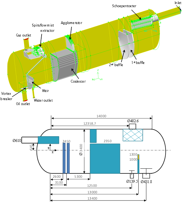Figure 1. Geometry and dimensions of the 1st stage separator

3. Mathematical Model

The unsteady turbulent multiphase flow was solved using the Reynolds averaged multiphase Eulerian-Eulerian and turbulence standard k-ε models implemented in the commercial code ANSYS Fluent 14.0[22]. As mentioned in the introduction, the k-ε model is a robust and simple turbulence model which provides the optimal performance in terms of accuracy and computational cost at the large scale of industrial applications. The mixture turbulence model is used in this study. The Eulerian-Eulerian model assumes mono-dispersed secondary phases represented by their average diameter and omits coalescence and breakup.

The model was found, in previous studies[19], to predict unrealistic results in terms of separation and entrainment of phases. It was necessary, hence, to use a more elaborate model to overcome the limitations of the Eulerian-Eulerian model. The Population Balance Model (PBM)[22] is thought to be the appropriate approach to account for the effects of the size distribution and the related complex phenomena such as breakup and coalescence[24] although limited to only one secondary phase. Furthermore, it has the advantage to be implemented as sub-model of the existing Eulerian-Eulerian multiphase model.

The general Eulerian-Eulerian model attributes separate momentum and continuity equations for each phase. Each momentum equation contains a term to account for the phase interaction. In the frame work of the Population Balance sub-model, an additional transport equation of the number density function (Equation 1) is solved for one of the secondary phases. Thus, the volume fraction predicted by the Eulerian-Eulerian model is divided into bin fractions for the phase represented by the PBM model. The additional PBM equation yields the local bin fractions and size distributions of the poly-dispersed secondary phase. Then, the resulting size distributions and bin fractions are converted to a mean Sauter diameter and a mean volume fraction to be implemented in the momentum equations of the other phases to account for the phase interaction.

(1)

In the present study, the Luo models for breakup[25] and coalescence[26] were used.

The Luo breakage model[25] is based on the idea of arrival of eddies of a spectrum length scales (frequencies) which causes the velocity, at the surface of a bubble or droplet, to fluctuate. These arriving turbulent eddies supply the necessary surface energy for the breakup of a particle.

(2)

is the arrival frequency of eddies of size (length scale) between λ and λ+dλ onto particles of volume V, is the modelled probability for a particle of size V to break into two particles, one with volume V₁=Vf_BV when the particle is hit by an eddy of size λ. f_BV is the Breakage volume fraction.

The arrival frequency of eddies with a given size λ on the surface of drops or bubbles with size d is equal to

(3)

is the number of eddies of size between λ and λ+dλ per unit volume and is the turbulent velocity of eddies of size λ[27].

For the breakage probability, and based on the probability theory, the probability for a particle of size V to break into a size of Vf_VB, when the particle is hit by an eddy of size λ, is equal to the probability of the arriving eddy of size λ having a kinetic energy greater than or equal to the minimum energy required for the particle breakup.

Referring to the literature on turbulence theory, e.g.,[27-29], each parameter is replaced by its appropriate formulation giving the final expression for the breakage rate

(4)

where .

(5)

ε is the turbulent energy dissipation rate

The Luo coalescence model[26], developed originally for bubble coalescence in bubble columns, suggests that the coalescence rate is a product of collision frequency and the coalescence efficiency.

(6)

Only binary collisions are considered since collision of more bubbles has a very small probability. The collision frequency , based on the approach of[30] for binary drop collisions in turbulent air, is a function of the bubbles velocities and diameters based on the assumption that the colliding bubbles take the velocity of the eddies with the same size, e.g.,[31].

(7)

For the coalescence efficiency , the idea is to compare the contact time t_I (interaction time based on the parallel film concept developed in the literature for equal-sized droplets and extended by[26] to unequal-sized droplets) and the coalescence time t_C.

(8)

(9)

(10)

(11)

The discrete method, of the PBM model[22], is used in the present work to generate a solution. It consists in representing the continuous size distribution as a set of discrete size bins. The advantages of this method are its robust numerics and the particle size distribution PSD which is calculated directly contrary to the method of moments. However, the bins must be defined a priori and a large number of classes may sometimes be required.

4. Simulation Approach

4.1. Boundary Conditions

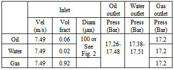
The boundary conditions, at the inlet and the outlets of the separator, are summarized in table 1. According to the inlet flow regime, a turbulence intensity of 2% was prescribed. The secondary phases (oil and water) were injected as mono-dispersed or poly-dispersed droplets in the continuous gaseous phase. Table 2 indicates the physical properties of the three phases which are assumed to be constant throughout the computational domain since the flow is treated as isothermal and incompressible. At the walls, no slip condition, with a standard wall function[22], was imposed. It removes the need for very fine meshes at the walls. It is believed that the dynamics of such a flow and scale are weakly governed by the presence of walls and hence the numerical errors induced by the choice of the standard wall function would have a negligible effect on the overall flow structure. A symmetry boundary condition was applied on the median plane of the separator in order to reduce the number of grid cells considering, thus, only half of the separator geometry. A pressure boundary condition was adopted at the outlets of the separator, as shown in Table 1. The pressure at the gas outlet was known while those at the liquid outlets were monitored to maintain the liquid levels and to ensure an overall phase mass balance.

Table 1. Boundary conditions

Table 2. Physical properties

4.2. Size Distribution

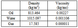
The size distribution used is represented by seven individual bins. Naturally, the accuracy of the discrete-phase PBM model might be improved with a higher number of bins, but with a penalty on the computational cost that has to be kept reasonable for any practical application.

The size distribution to be used at the inlet can be assumed to be normally distributed using the Rosin-Rammler function[22].

(12)

Y_d is the mass or volume fraction of the droplets which diameter is greater than d.

The Rosin-Rammler approach requires two parameters which are the mean diameter and the spread parameter n.

In the literature, details on size distribution for gas/oil/water mixtures, at this stage of separation, are scarce. Hallanger et al.[21] mentioned a mean droplet diameter of 250 μm with a standard deviation equal to 3 estimated from a correlation based on data from some North Sea oilfields. They divided their distribution into 7 groups. Hansen and Rørtveit[5] in their simulations assumed a distribution with an average diameter equal to 166 μm with a minimum of 75 μm and a maximum of 316 μm. Laleh[32] constructed a size distribution based on the approach of the maximum stable diameter which is estimated based on fluid properties and flow characteristics. After calculating the maximum stable diameter using several correlations existing in the literature, Laleh[32] opted for a distribution with a maximum diameter equal, approximately, to 2000 μm and 3700 μm for oil and water respectively under the conditions of low operating pressure (0.7-2.7 bars) and a Reynolds number larger than 2300. The minimum diameter for both phases was 100 μm.

For the spread parameter n (see Equation 12), Laleh[32] used an average value of 2.6 extracted from experiments [33-34].

Furthermore,[1] stated that, in the absence of laboratory or field data, water droplets of diameter larger than 500 μm should be separated leading to 10% of water or less to be lost with the oil phase. In terms of gas-oil separation, the design oil droplet diameter recommended by the Literature[1] is in the range 100-140 μm. Relying on the limited information from the literature, a spread parameter of 2.6 and three average diameters (150, 500, 800 μm for water and 50, 80, 140 μm for oil), were used in the present study. When oil was the poly-dispersed phase (Figure 2.a), water was represented by a 400 μm mean diameter mono-dispersed distribution while when water was the poly-dispersed (Figure 2.b) phase, oil was represented by a 100 μm mean diameter mono-dispersed distribution. The water poly-dispersed distributions were meant to compare an arbitrarily skewed distribution with two normal Rosin-Rammler ones (Fig. 2.b). It is important to mention that the Previous Eulerian-Eulerian simulations were conducted with mono-dispersed oil and water phases which average diameter was equal to 100 μm. Other simulations, not shown here, were conducted with different mean diameters and led to different entrainment amounts indicating the necessity to employ appropriate models to include poly-dispersed distributions, with coalescence and breakup, rather than mono-dispersed ones.

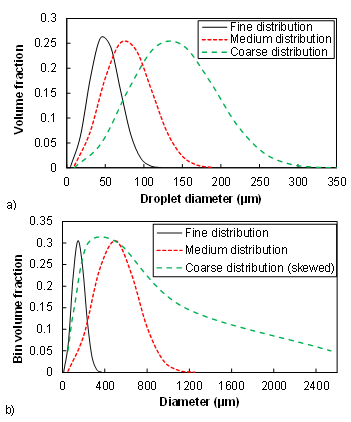Figure 2. Volume fraction vs droplet diameter. top) oil, bottom) water

4.3. Simulation Strategy

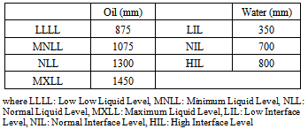
The PBM model simulations were initiated using a developed flow resulting from previous simulations with the Eulerian-Eulerian model[18-19] for a more rapid convergence of the solution.

The convergence of the transient simulation was based on the decrease of the residuals by at least three orders of magnitude as recommended by ANSYS FLUENT[22]. In terms of temporal convergence, the simulation using the PBM model exhibited a quasi-steady flow behaviour, with no temporal variations of the flow rates at the three outlets of the separator and no noticeable changes of the overall size distribution, after about 1200s (20 minutes).

Subsequent to the transient simulation, the average field properties were calculated during about 600s in a quasi-steady regime. The transient flow duration corresponds to the approximate design residence time recommended in the literature which ranges between 1-3 minutes for the gas-liquid separation and 3-30 minutes for the liquid-liquid separation[1]. The liquid levels were maintained in the limits presented in Table 3.

Table 3. Characteristic liquid levels

The simulations, necessitated 30 days of continuous run to simulate 20 minutes for the transient period and additional minutes for the calculation of the mean field properties of real time on 48 parallel processors of a High Performance Cluster.

5. Results and Discussion

The droplet size distributions considered are expected to affect both the overall performance of the separator and the internal flow behaviour. The performance, predicted by the PBM model, is compared with the Eulerian-Eulerian simulations[18-19] and ADCO field test results. It is worth mentioning that the field tests accuracy is debatable due to the difficulty of obtaining rigorous measurements of such multiphase flows. The main differences between the two approaches, Eulerian-Eulerian model with and without PBM, are expected to manifest in terms of water-in-oil and oil carryover parts of the phase separation process as the water-in-gas and oil-in-water were found to be negligible from the field test results and the previous simulations. The flow field behavior is further validated by semi-empirical results from the literature in terms of residence time and settling velocity. Finally, the size distribution is tracked at different locations inside the separator for a deeper investigation of the local effect of the internals on the injected droplet populations.

5.1. Performance

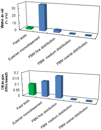Figure 3. Entrainment rate in field units: top) water-in-oil, bottom) oil-in-gas. USG: United States Gallons, mmcf: million cubic feet

Figure 3 presents the amount of water entrained by the oil and the amount of oil carryover towards the gas outlet when water and oil were assumed poly-dispersed respectively. It is clear that the Eulerian-Eulerian model, without PBM, overestimates the water-in-oil amount considerably due to the unrealistic mono-dispersity assumption and the omission of coalescence and breakup where the predicted value by CFD is about 17 times that of the field tests. However, the PBM model predictions are reasonable within the range of droplet size distribution considered. The fine distribution generates slightly higher water-in-oil entrainment (50%) compared to the field tests while the medium and the coarse distributions almost eliminate the entrainment completely. Similar results were obtained for the oil carryover with overestimations equal to 33% and 85% for the Eulerian-Eulerian simulations and the PBM fine distribution respectively. Injecting larger droplets such as those of the medium and the coarse distributions reduced the oil carryover to negligible values. Thus, it would be interesting to test an intermediate size distribution between the fine and medium ones to determine which distribution would yield an oil-in-gas amount comparable with the field test results.

5.2. Residence Time

Several previous studies discussed the estimation of the residence time distribution RTD and the mean residence time MRT, e.g.,[35-36], among which few were devoted to oil/water gravity separators, e.g.,[8,10-11]. The studies were based on the concept of tracer injection. Danckwerts[35] stated that the MRT can be estimated simply from

(13)

where V is the volume occupied by the phase and is the flow rate of the same phase at the inlet of the separator.

Livenspiel[36] proposed a semi-empirical formula (Equation 14) to estimate the MRT based on the RTD obtained from experiments where a fixed quantity of oil-soluble and/or water-soluble tracers were injected at the inlet of the primary oil/water separators[8]. Measurements of the tracers’ concentrations with time, at the outlet of the separators, yielded a bell-shape distribution characterized by a first sign of entrainment (increasing concentrations starting from zero), a peak, and a slope towards zero corresponding to the last traces of the tracer.

(14)

where c(t) is the tracer concentration at the corresponding outlet of the separator.

The mean residence time MRT is plotted in Figures 4.a and 4.b. The MRT for the gas-liquid separation (Figure 4.a) exhibits a decreasing trend with increasing mean diameters of the inlet size distributions which is caused by the rapid settling of the larger droplets. The simulation values are three times larger than those recommended by standards[37] and about 40% lower than Arnold and Stewart method. Machado et al.[38] used the tracer technique to measure the MRT for gas-liquid separation in a battery of three separators operating in serial mode. Although the dimensions of the separators were not mentioned, their MRT values obtained by experiments and simulations are reported in Figure 4.a and are comparable to the API12J recommended values.

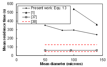Figure 4.a. Mean residence time vs mean droplet diameter: gas-liquid separation

For the liquid-liquid separation, Simmons et al.[8] obtained MRTs for different separators operating in different fields under, slightly, different operating conditions from the present study using Equations 13 and 14.

The inlet flow rates were close to those used in the present work. The separators had the diameter x length dimensions as follows: 3.6x24.5m, 3.05x12.3m, 3x9.9 m, 3.3x9 m, and 2.64x7.4 m. Some of the cases contained a layer of sand in the bottom of the separator affecting the characteristic interfaces levels. Some of these results are illustrated in Figure 4.b for comparison with the results of the present study obtained from Equation 13.

A modified Stewart and Arnold[1] method for appropriate separator sizing was proposed by Boukadi et al.[39]. It implements the appropriate emulsion viscosity and flow rates in the classical correlation of the terminal velocity derived from Stokes Law based on a design droplet diameter equal to 200 μm for the gas-liquid separation and 500 μm for the liquid-liquid separation. It is worth to mention that the abovementioned design methodologies are all based on a cutoff diameter of 100-140 μm for oil-gas separation and 500 μm for oil-water separation. They compared the residence time values obtained from[37], Stewart and Arnold method, and their modified approach focusing on the liquid-liquid separation. The values are reported in Figure 4.b. Significant discrepancies can be seen between the present simulation results and the classical API method. However, Boukadi’s improved method agrees with the CFD results for the design droplet diameter of 500 μm. The simulation results are in a good agreement with Arnold and Stewart method with a discrepancy in the order of 20%.

Although, the improved method of[39] employed more realistic parameters (more realistic flow rates and emulsion viscosities) compared to the classical design approaches, CFD is the only approach susceptible to account for all the parameters affecting the performance of the separator especially the effects of the internals usually approximated through the K-factor in the settling velocity equation or omitted completely in the other methods.

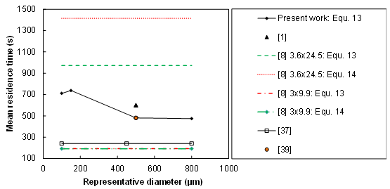Figure 4.b. Mean residence time vs mean droplet diameter: liquid-liquid separation

5.3. Velocity Field

Since the multiphase flow is governed by the principal of settling, based on the Stokes law, it is worth exploring the fields of the horizontal and vertical velocity components. Representative horizontal and vertical lines (Figure 5), on which profiles of the horizontal and vertical velocity components are plotted in figures 6 and 7, were placed 0.3 m away from the plane of symmetry. One important observation is that the separator internal volume can be divided into distinguished regions according to the phase volume fraction, i.e., for the oil, for example, the internal volume can be divided into three regions which are: the gas-rich upper part where the oil is present with relatively low fraction and has, hence, the same velocity as the gas stream, the oil-rich layer, and the water-rich lower part where the oil is almost entrained by the water stream and has the same velocity. Based on this fact, it was considered that Figure 6 could describe the behavior of all the phases in the axial direction.

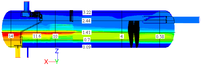Figure 5. Horizontal and vertical lines used to plot the velocity components superimposed on contours of oil volume fraction

At x=0.58m, inside the Schoepentoeter, there is a core flow with high positive axial velocity surrounded by two reverse streams. Underneath the Schoepentoeter, the axial velocity exhibits a decaying trend until the bottom of the separator. Above NLL, at x= 4m and x=10m, a slight acceleration, with axial velocities not exceeding 1m/s, are caused by the presence of the baffles, the coalescer, and the agglomerator.

The Spiraflow mist extractor (x=11.6 m) is found to generate very high axial velocities in the range 12-18 m/s. This can be explained by the reduced open area of the Spiraflow which represents almost a quarter of that of classical vane pack types.

Profiles of the oil and water vertical velocity components, along axial lines at different horizontal positions, are presented in Figures 7.a and 7.b respectively.

Due to the low values of the vertical velocity component close to the bottom of the separator from the mixing compartment, upstream of the first baffle, until the weir position, they were multiplied by 50 for the position z=0.09m and by 10 for the position z=0.4m respectively. Downstream of the weir, the values were not changed. At z=0.09, the horizontal line is submerged in the water layer. The baffles dampen the perturbation of the flow generated by the inlet stream. Upstream of the coalescer, at x≈8.5m, the flow contains almost only water. The flow becomes disturbed by the effect of the coalescer which seems to cause some oil to be entrained downward.

At the bottom of the oil layer, z=0.7m, the flow is stable in the vertical direction and only a negative peak is seen downstream of the weir (at x=13m) due to the spillway effect. At the top of the oil layer, z=1.41m, the flow is stabilized, with negative z velocities, under the effect of the baffles but slight perturbations are generated by the coalescer. The spillway behavior is no more present.

At z=2.44m, crossing the inlet device, the Schoepentoeter causes the flow to have a downward/upward sinusoidal-like trend. Beyond the inlet device, no settling of the oil is seen (Figure 7.a) while the heavier water phase undergoes a relatively important settling behaviour (Figure 7.b). The settling behavior is slightly enhanced at x≈8.5m (agglomerator location).

At the top (z=3.22m), apart from the inlet region and the mist extractor devices, no noticeable liquid settling or entrainment is observed. Again, the accelerations inside the Spiraflow are higher than elsewhere.

The settling velocity can be represented by the negative vertical velocity component which contours, superimposed with streamtraces, are plotted in Figure 8. The range of values plotted is limited to -0.05÷0m/s for display purposes only and the appropriate values in the positions mentioned will be cited explicitly in the text. The streamtraces are intended to show the flow direction at different locations of the separator.

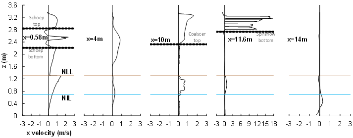Figure 6. Profiles of axial oil velocity component plotted on vertical lines at different axial positions. The values underneath NLL are multiplied by 10. The dashed lines represent boundaries of internals

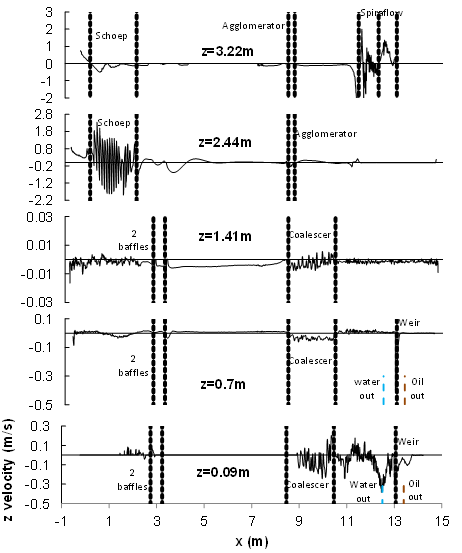Figure 7.a. Profiles of vertical oil velocity component plotted on horizontal lines at different vertical positions. The dashed lines represent boundaries of internals

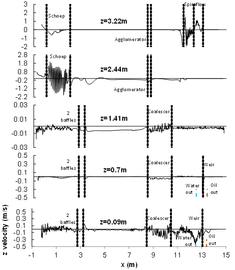Figure 7.b. Profiles of vertical water velocity component plotted on horizontal lines at different vertical positions. The dashed lines represent boundaries of internals

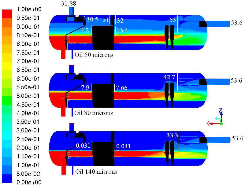
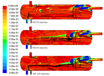Figure 8. Negative oil z velocity (m/s) distribution in the symmetry plane

Towards the Shoepentoeter outlet, the vertical component is about -2.5m/s for the three cases which should aid the early droplet settling. In the mixing compartment (upstream of the baffles underneath the Schoepentoeter), the larger are the droplets the higher is the settling velocity. Immediately downstream of the baffles, another region with very high settling velocities can be seen with values reaching 2m/s for the medium and coarse distributions.

This region of high settling velocities extends until the coalescer. The fine distribution, expected to cause more entrainment, contains slightly high settling velocities near the top of the separator in the settling compartment meaning that the fine droplets reached very high positions contrary to the other distributions with larger droplets. This is confirmed by the horizontal streamtraces directed towards the Spiraflow. For the medium and coarse distributions, the streamtraces, within the gas compartment, are directed downwards due to a more pronounced settling effect especially downstream of the baffles. Recirculation zones are observed for the medium distribution within the oil layer which agrees with results from the literature[5].

The settling velocity was noticeable in a limited region of the settling compartment. Representative values, within this region, are compared with values extracted from the theoretical Stokes law in Figure 9.

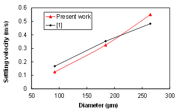Figure 9. Oil settling velocity vs representative droplet diameter

The representative diameters, for the simulation results, correspond to the largest droplet since it was found that it is the predominant size in the settling compartment (see section 5.4). The CFD results are in good agreement with the theoretical values with a discrepancy of about 25%. However, CFD provided a full description of the settling velocity field while the semi-empirical approach considered a representative value in the settling compartment. Such more complete view of the flow field is very important and should be helpful for the design of more efficient separation devices.

The positive vertical component represents the rising velocity and is useful to describe the oil-in-gas entrainment and the rising of the oil droplets within the water layer towards the oil-water interface (Figure 10). The range of values plotted is limited to 0-0.1 m/s for display purposes only and the appropriate values in the positions mentioned will be cited explicitly in the text.

It can be seen that the first region with important oil entrainment is located underneath the Schoepentoeter in the mixing compartment. Here, values reaching 0.1-0.15 m/s were noticed. In the settling compartment, the rising velocity (oil entrainment) persists only in the case of the fine distribution and slightly for the medium distribution. Within the water layer, rising velocities in the settling compartment were equal to 0.01, 0.015, 0.02 m/s for the fine, medium, and coarse distributions respectively. This is in agreement with the well-known behavior of oil droplets in stratified oil-water flow. The high rising velocities persist until the coalscer with higher values for the larger droplets.

For the water phase, the negative vertical-component velocity (Figure 11), superimposed with streamtraces, is plotted with a range of values limited to -0.05÷0 m/s for display purposes only and the appropriate values in the positions mentioned will be cited explicitly in the text. Within the gas compartment, a region with very high settling velocities (-0.5 m/s) extends in the axial direction and reaches the coalescer for the fine distribution while shrinks backwards for the two other distributions. Within the oil layer, the settling velocity is very high upstream of the baffles and decreases in the axial direction. Within the oil layer downstream of the baffles, the water settling velocity is negligible for the fine distribution which justifies the entrainment discussed in section 5.1 whilst it persists for the two other distributions which explains the perfect separation in these cases.

The descending streamtraces illustrate the important settling effect within the mixing and settling compartments. The horizontal streamtraces, within the oil layer for the fine distribution, characterize the entrainment of water with oil.

Figure 12 compares the water settling velocity extracted from CFD and Stokes law in the settling compartment with the same approach explained for Figure 9.

The CFD results are lower than the theoretical values with a discrepancy of about 43 %.

The rising velocity for the water phase (Figure 13) is marginal in almost the whole domain.

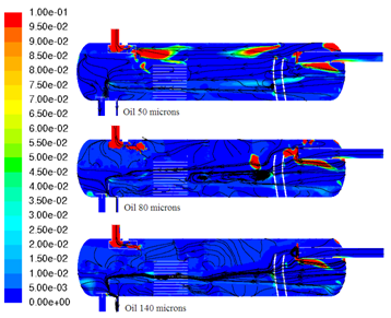Figure 10. Positive oil z velocity (m/s) distribution in the symmetry plane

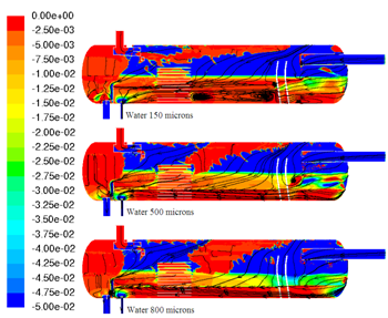Figure 11. Negative water z velocity (m/s) distribution in the symmetry plane

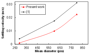Figure 12. Water settling velocity vs representative droplet diameter

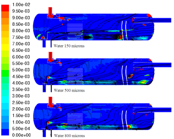Figure 13. Positive water z velocity (m/s) distribution in the symmetry plane

5.4. Effects of the Internals

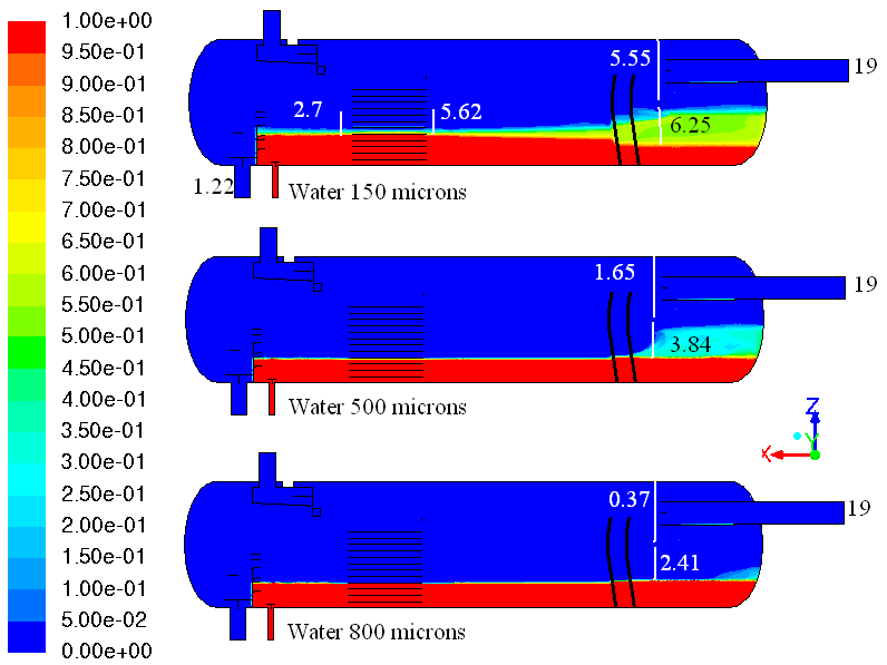
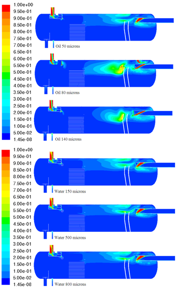
The total amount of the entrained oil or water, in addition to the local droplet size distribution, were tracked at different locations inside the separator to assess the effects of the internals (Figures 14-15 for the oil phase and Figures 16-17 for the water phase).

The amounts of entrained phases (Figures 14 and 16) illustrate the separation performance of the individual internals while the size distributions tracked in Figures 15 and 17 explain the impact of the locally-generated population on the separation performance.

Figure 14. Contours of the oil volume fraction in the symmetry plane. The white vertical lines indicate- the planes created to quantify the amount of entrained phase in kg/s

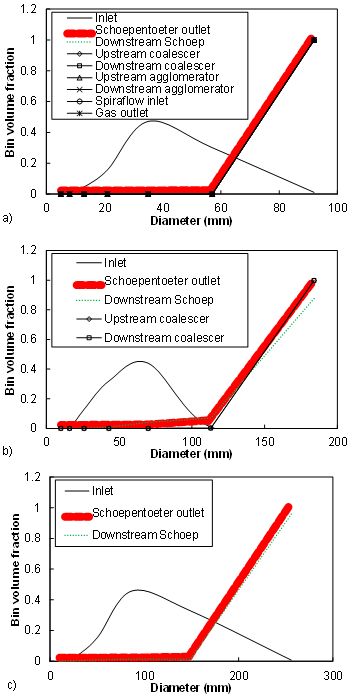Figure 15. Oil droplet size distribution at different locations inside the separator: a) Fine distribution, b) Medium Distribution, c) Coarse distribution

Figure 16. Contours of the water volume fraction in the symmetry plane. The white vertical lines indicate- the planes created to quantify the amount of entrained phase in kg/s

5.4.1. Schoepentoeter

Viteri et al.[40] mentioned that the Schoepentoeter separates 60-70 % of the incoming liquid but nothing has been mentioned about the assessment approach and how the separation efficiency was estimated. Mosca et al.[41] explained briefly that the Schoepentoeter efficiency was estimated based on the information upstream (inlet) and downstream (column diameter of vertical separator) which is similar to what was done in the present study by creating a plane crossing the gas layer immediately downstream of the Schoepentoeter.

From Figures 14 and 16, it can be noticed that the schoepentoeter efficiency is sensitive to the initial droplet size distribution.

The schoepentoeter plays a key role in coalescing small droplets into larger ones. In fact, Figures 15 and 17 illustrate the size distribution at the inlet (Rosin-Rammler) and the Schoepentoeter outlet (mainly the largest size). For the fine oil distribution (Figure 15.a), all the 6 smaller droplet sizes disappeared forming a mono-dispersed distribution at the Schoepentoeter outlet, and the plane downstream of it, with a diameter equal to that of the largest droplets (92 μm). However, Figure 14 shows that almost no separation has taken place within the separator as the amount entrained by the gas is almost equal to that at the inlet. This suggests that the separator is designed to separate droplets larger than 92 μm while the fine distribution of the PBM model is limited to the maximum imposed a priori.

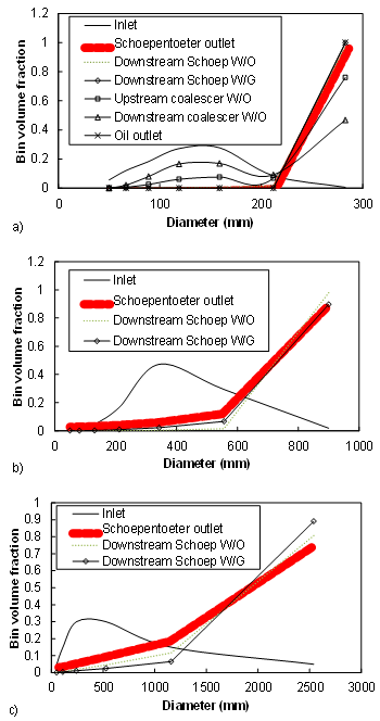Figure 17. Water droplet size distribution at different locations inside the separator: a) Fine distribution, b) Medium Distribution, c) Coarse distribution

For the medium oil distribution, the Rosin-Rammler inlet distribution becames a quasi-mono-dispersed distribution at the Schoepentoeter outlet and downstream plane although few percent of smaller droplets still exist. It can be said that the Schoepentoeter eliminates all the droplets smaller than, approximately 50 μm.

The Schoepentoeter contains several lateral flow passages with guiding vanes that change the momentum of the incoming flow by changing the flow path to generate a centrifugal force component that enhances liquid droplet separation being ejected towards the outer wall of the diffusers. Polderman et al.[42] mentioned that the Schoepentoeter may promote coalescence under the effect of centrifugal acceleration. Figure 17 shows that the trend for the water phase is identical with the droplets smaller than 200 μm being almost completely eliminated under the coalescence effect in the Schoepentoeter. Hence, the Schoepentoeter duty is to separate a major part of the inlet stream and to generate coarser droplet size distribution, by coalescence, susceptible to be separated efficiently in the downstream region.

5.4.2. Coalescer and Agglomerator

Rommel et al.[43] conducted experiments to develop a methodology for plate separators design (coalescer). They investigated the effects of the plate inclination, the plates spacing and the dispersed phase load on the plates’ separation efficiency. They stated that the plate separators are usually operated at inclination angles equal to 15°. In our case the inclination angle is equal to 60°.

The distribution at the inlet of the coalescer, generated by the upstream internals (Schoepentoeter and baffles) is mono-dispersed for the oil phase (Figure 15) while quasi-mono-dispersed for the water phase (Figure 17) with diameters corresponding to the largest size for each distribution which is really the maximum attainable size defined by the PBM distributions imposed.

The water-in-oil dispersed load in the present study lies within the ranges tested by the authors. Under the flow Conditions of the present study upstream of the coalescer, the expected separation efficiency should be less than 95% according to Rommel et al.[43]. In the present study the separation efficiency of the coalescer is equal to 52% for the separation of water droplets from oil (fine distribution).

The volume fraction of droplets, smaller than 200 μm, increases through the coalescer while that of droplets larger than 200 μm decreases. This can be explained by the fact that large droplets are more susceptible to gravity settling effects.

At the oil and water outlets, the droplets smaller than 200 μm disappeared due to coalescence in the space separating the coalescer outlet and the separator liquid outlets.

Concerning the separation of oil droplets from gas, it was found that the coalescer contributes with a separation efficiency equal to 70% for the oil fine distribution while inefficient for the coarser distributions. The agglomerator was involved in the separation process only for the case of oil droplets with fine distribution. The simulation results predicted very low separation efficiency which cannot be confirmed or rejected due to the absence of reliable data for comparison.

5.4.3. Spiraflow

The fine oil distribution is the only case where the liquid reaches the gas outlet (Figure 14). The corresponding size distribution, in the gas outlet region is presented in Figure 15.a. It was found that the entire amount entering the spiraflow is leaving through the gas outlet with zero separation efficiency. Kremleva et al.[44] stated that the Spiraflow separation efficiency should be 99.99% when the liquid volume fraction doesn’t exceed 0.05. In the present study, the oil volume fraction, at the inlet of the Spiraflow, was 0.055. Thus, the discrepancy might be due to several causes among which the unknown, and hence approximated, internal geometry might be the major source.

In addition to the interesting phenomena related to the effects of the internals on the multiphase flow behaviour for different size distributions, Figures 14 and 16 show noticeable diffusion bands nearby the characteristic interfaces. From Figure 14, it can be seen that an oil-reach layer form above the gas-liquid interface, for the fine and medium distributions, which should correspond in practical cases to foaming. From Figure 16, another diffusion band is formed at the liquid-liquid interface level. It was found in the literature[6-7] that similar phenomena are not unexpected in such facilities. However, a deeper investigation is required to quantify the characteristics of these diffusion bands.

It is worth mentioning that no noticeable breakup effects were observed for the cases considered. The separator, with the upgraded internals, is meant to minimize the shearing effects generated by the old internals[18-19]. Thus, if breakup occurs in the upgraded separators, it is expected to be important through the perforated baffles. Unfortunately, the baffles, in the present study, were represented by porous media which cannot replicate the shearing effects generated by the holes of the real baffles in an appropriate way. Indeed, it was explained that the velocity increases locally through the holes increasing, hence, the turbulence and shearing rates and promoting the breakup effect[9].

5.5. Turbulence Field

Figure 18 illustrates the turbulent kinetic energy contours in the plane of symmetry. The maximum turbulent kinetic energy, for all the cases, is equal to about 6 m²/s². However, the values were limited to 1 m²/s² for a clearer display. It is clear that the Schoepentoeter and the Spiraflow generate the highest turbulence levels due to their complex geometries and the high velocities they engender (see Figure 6). The space above the baffles is also seen to generate high levels of turbulence because it creates a sudden contraction effect. This might disturb the plug flow required for an efficient separation and increase the probability of the entrained droplets breakup. Within the liquid layers the turbulent kinetic energy is negligible thus enhancing coalescence. The most noticeable difference, between the cases considered, is that the turbulence-affected area, when oil is the poly-dispersed phase, is more noticeable for the medium and coarse distributions especially downstream of the baffles and upstream of the Spiraflow. It should be mentioned that the region downstream of the baffles is characterized by an important settling of the oil droplets especially for the medium and coarse distributions (Figures 8 and 14). However, when the water is the poly-dispersed phase, almost all the droplets are separated within the mixing compartment upstream of the baffles which explains the identical turbulence field for the three distributions.

Figure 18. Contours of the turbulent kinetic energy in the symmetry plane.

6. Conclusions

The Population Balance Model (PBM), in conjunction with the Eulerian-Eulerian model, was used to simulate the complex multiphase flow in a horizontal separator. The study focused on the effects of the size distribution of the secondary phases on the performance of the separator and the internal flow behavior. Three secondary phase distributions were used based on values recommended in the literature for design purposes.

The three distributions, referred to as fine, medium, and coarse, were found to be differently affected by the internals. Their predicted effects were in a fair agreement with the scarce data ranges existing in the literature; namely, ADCO field tests and the semi-empirical approach based on Stokes law.

Overall, both oil and water as poly-dispersed secondary phases lead to better separation efficiencies. As expected, it was found that the schoepentoeter plays a major role in initiating droplet coalescence and deserves further investigation. Indeed, the flow at its exit displays a quasi-mono-dispersed distribution. Downstream, the size distribution remains unchanged throughout the whole remaining liquid path inside the separator. The coalescer was found to contribute for the fine distribution only. Coalescence was found to be crucial for the correct prediction of separation efficiency.

In terms of mean residence time MRT, finer distributions generated higher MRTs. The simulation results were comparable to existing experimental and semi-empirical data from the literature.

The present study highlighted the importance of the droplet size distribution in accurately predicting the performance of the separator and the internal multiphase flow behavior. Inversely, when the overall performance is known a priori from experiments or field tests, the PBM approach is useful for the prediction of the appropriate size distribution, at the inlet of the separator. The results of the present study showed that the PBM model, with an additional equation for the transport of number density function, represents a noticeable improvement over the limited standard Eulerian-Eulerian model with no additional computational cost.

The results of the present study can be further refined by implementing the real configuration of the baffles instead of the porous media model used but with a heavy penalty on grid size and computational time. Although taking into account breakup and coalescence, the PBM model still imposes a priori limitations on the size distribution. Future studies could consider a more elaborate turbulence model such as Large Eddy Simulation since the PBM model relies on the predicted turbulence field to replicate the breakup and coalescence phenomena more accurately.

ACKNOWLEDGEMENTS

This study was funded by Abu Dhabi Company for Onshore Oil Operations (ADCO). The technical support from the engineers of ADCO is gratefully acknowledged.