1. Introduction

The family of classical self-oscillatory flows containes supersonic flows near blunted bodies with front projections, flows with supersonic jet inflowing to a cavity (Hartman whistle), the flows with supersonic jet running at the infinite or finite plane surface. This paper is devoted mainly to investigation of the self-oscillations mechanism in flows of this family and to inclusion of new unsteady flows to it. Search of new self-oscillatory flows is carried out here and in[1-4] on a base of the hypothesis of self-oscillations mechanism , proposed in[5]. This mechanism supposes availability of “active” elements of flows, namely, elements, which amplify disturbances. Supposition is used about two types of “active” elements – contact discontinuities and intersection points of shocks with shocks or shocks with contact discontinuities. Possibility of the disturbances amplification by contact discontinuities is a result of the Kelvin-Gelmgoltce instability and is accepted. Inclusion of intersection points to a list of amplifiers is proposed in[13]. It is initiated by known possibility to operate types of the shock reflection from plane surface (Mach or regular types) by small influences. If small influences yield significant change of the flow in the reflection zone, that means that this flow structure is an amplifier of disturbances. Possibility of total intersection points of discontinuities (intersection lines in 3d case) to amplify disturbances should be an object of additional investigations and is used here as a supposition, which is checked by results of the search for new unsteady flows.

Since active flow elements, mentioned above, amplify disturbances, that means, that these elements may interact one with another. Namely, disturbances from one element affect at the flow near some another. Change of the flow near the last element affect at the flow near initial one. If the reflected disturbances come back to initial element with nearly the same phase, as this element is emitting at that moment, then conditions are formed for the positive feedback effect. As a result, a resonance may take place, which induces self-oscillations of the flow. Availability of these ‘active’ elements does not guarantee producing of self-oscillations and may provide existence of steady flows with normal or large time, necessary to get steady state.

There is possibility of three type of interaction:

1 - contact discontinuity with contact discontinuity;

2 - intersection point with contact discontinuity;

3 - intersection point with intersection point.

The start of our numerical study[9-11] is made under supposition, that second type is most active in producing self-oscillations. Bat next investigations [12] show; that third type of interaction induces more intensive self-oscillations. Here this conclusion is illustrated by next numerical investigations.

2. Mathematical Model

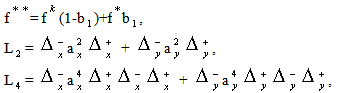
Both Euler equations and Reynolds equations added by differential or algebraic models of turbulence are usually employed in investigations of self-oscillatory flows[3-8, 14]. It seems that usage of Reynolds equations for a search for new unsteady flows is preferable. The matter of fact is that the Kelvin-Helmgoltce instability of contact discontinuities makes studied problems mathematically incorrect. Usage of the turbulent viscosity allows to make it correct and to achieve convergence of solutions by the number of mesh points. If calculations of previously experimentally investigated unsteady flows may be verified by comparison of obtained results with known data, convergence of solutions by number of mesh points is really the only criteria of reliability of obtained numerical results in a search for new self-oscillatory flows.

Thus, Reynolds equations and a turbulence model, similar to Cebeci-Smith model[13], are used. The length scale in this model is defied as a thickness of the local shear layer; at the same time, since algebraic formulas yield acceptable results mainly for small scale oscillations, the calculated scale is limited somewhat by the small value. This approach is closed technically to algebraic versions of approach LES (Large Eddy Simulation, see, for example,[14]), but there is principal difference of the used approach and LES. The mesh cell size is used as the length scale in algebraic versions of LES[14]. It allows to describe lesser pulsations when the mesh number increases, but prevent checking of solutions convergence by the number of mesh points, since varying of this number yields varying of turbulent viscosity. Used here approach deals with the fixed aggregate of scales of disturbances represented in the turbulent viscosity. As a result, the turbulent viscosity and, consequently, the thickness of a contact discontinuity (more precisely, shift layer in our case) are steady while the mesh number is varying.

Since Kelvin–Helmholtce instability of a contact discontinuity plays important role in resonance processes, producing self-oscillations, the numerical method should provide good resolution of contact discontinuities. It may be noted that numerical methods smear excessively (much more than shock waves) long contact discontinuities, since the "gradient catastrophe" phenomenon is not true for these discontinuities ("gradient catastrophe" phenomenon consists in a "steeping" of compression waves). To eliminate this negative smearing high order schemes may be used. The implicit conservative Runge-Kutta scheme[15-16] is employed here, which is third order in time and fourth order in space variables (viscous terms are approximated with second order).

The used numerical method is shown below for the case of zero viscosity, Cartesian system of coordinates and omitted adaptation algorithms. 2D system of gas-dynamic equations is written in the form

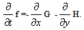(1)

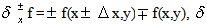
If to use designations equations (1) may be written with fourth order of approximation as a system of ordinary equations

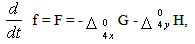
/6).

The intermediate form of the scheme consists of next two steps

(2)

(3)

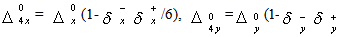
where =DG/Df, =DH/Df are Yacoby matrices, =|u|+c, =|v|+c - spectral radiuses of these matrixes,

Stability operators are factorized approximately to get each factor with space finite difference derivatives in only single variable. Then these operators are inversed by recurrent exclusion procedures. The absolutely stable third order method is provided by next values of parameters

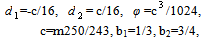(4)

where m=2 – number of space variables. The implicit first order scheme, determined by parameters

is also used in calculations (other parameters are calculated by formulas (4)). It should be noted, that the second step (3) is necessary for the third order scheme to satisfy both conditions of stability and approximation, more over, it provides conservativeness of the scheme. This second step is necessary only to provide conservativeness of the first order scheme. Numerical results for both schemes are in satisfactory agreement. Viscous terms are approximated for both schemes by second order weighted formulas with weights 0.5 at new and old time levels.

As mentioned above, the turbulent viscosity is important part of numerical method. To calculate it the algebraic turbulence model, similar to the Cebeci–Smith model, is used. The viscosity calculation starts with the determination of mixing layers by the calculation of a vorticity. The current mesh cell belongs to any mixing layer if wS=∑(u∆r) ≥ ε∆ξ ∑|u||∆r|, where w is a vorticity, S is an area of the mesh cell, ∑ is a sign of summation over cell sides, u are velocity vectors at mesh nodes, ∆r are vectors connecting neighbouring nodes, ε is the small constant (for which the value 3/N is choosed in trial calculations, N- the most number of mesh points along of space variables). The sum at the left side approximately represents the velocity circulation along the contour of the mesh cell. Similarly to the Cebeci-Smith model, the Prandtl formula µ=ρ|w|z² is used for the viscosity inside the mixing layer, where ρ is the density and z is the length scale, which is calculated by next formulas:

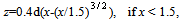z=0.4d, if x>1.5, x=L/d.

Here L is the distance from the current point till the mixing layer boundary, d is the delimiting parameter, which makes possible to present in the turbulent viscosity only short wave pulses, while the remainder are described by the mesh solution. These formulas are received from the Karman formula z=0.4L, which is used in the Cebeci-Smith model. Formula z=0.4min(L,d) was used in[9-13]. Formulas above describe the more smooth (first derivative is continuous) delimiter. This procedure is more correct, while numerical results change negligibly. Calculations, presented here, are carried out for d=r/60, r – radiuses of spherical blunts of considered bodies or the jet radius in investigations of supersonic jets impinging on plane.

Naturally, numerical calculations deal with dimensionless variables. These variables are defined as relations of initial variables and next parameters of the undisturbed flow or body size: - for pressure, - for density, - for velocity, r (blunt radiuses of cones or cylinders) – for space variables, r/ - for time. It is necessary some units of the dimensionless time to get steady state of usual flows. Here numerical modeling of flows is carrying out for tens and hundreds units. Necessity of usage of long time intervals is explained by slow definition of self-oscillatory flows structures.

3.Two Classical Self-oscillatory Flows

To check the numerical method and turbulence model the cavity flow [17] is calculated. Cavity ( Figure 1a) has depth D=5.2mm, length L=10.4mm, cavity grid contains 280 x 211 unifirn rectangular cells. Numerical region above cavity has height 10.4mm, length 20.8mm, and contains grid 561 x 322 with rectangular cells of the same length and of the variable height, increasing when distance from body surface increases. This cavity is tested numerically with flowfield conditions =2, θ=0.979mm (momentum thickness of the bound layer at beginning of the region above cavity). Boundary conditions for the computation are no-slip adiabatic wall on solid surfaces, extrapolation on the outflow boundaries, prescribed variables on the inflow plane. 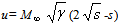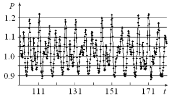Namely, dimensionless pressure and density are 1, velocity component v normal to wall is 0, velocity component tangential to wall is if s=y/θ≤10, u=, if s=y/θ >10, γ – specific heat ratio.

Calculations are carried out with a time step such that the maximum Courant-Friedrichs-Lewy (CFL) is 0.97. Figure 1b shows pressure history at the x=2L/3 point on the cavity floor. One time point of every 75 points is represented in figure 1b.

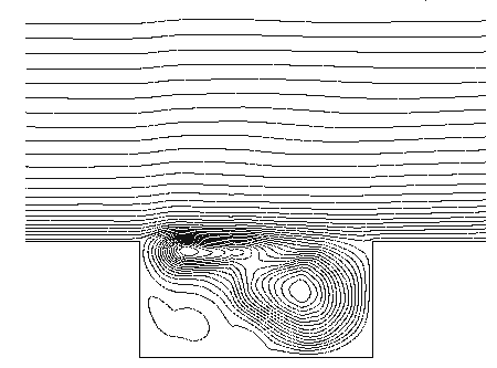Figure 1a. The cavity flow streamlines

Figure 1b. Time pressure history on the cavity floor

The time history of the surface pressure is used to form the time averaged sound pressure level , which is computed by the equation

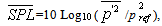where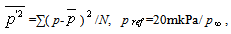

=98066Pa (the air pressure air under normal conditions) is used since dimensionless variables are dealt here. The resulting time averaged of 174.8Db may be compared with numerical of 167.54Db and experimental of 164.41Db presented in [17]. Weighted for data from various sources[18] is approximately 171Db.

Underexpanded supersonic jet impinging on plane is well studied experimentally and may be used to verify applicability of the described numerical method and turbulence model for study of self-oscillatory flows. It may also illustrate the proposed self-oscillations mechanism. Figure 2a shows the density distribution between two infinite plane surfaces. The jet outflows from the axisymmetrical nozzle at the left plane surface in figure 2a. The supposition is used that the temperature at center of the exit cross section of the nozzle is equal to the temperature of surrounding air. Jet parameters are computed by the system of algebraic equations, which describes one-dimensional flow from the point source. Velocity components normal to the solid surfaces (vertical boundaries in figure 2a) are equal to zero, tangential component of velocity, pressure and density are extrapolated. Radial component of velocity is equal to zero on symmetry axis, other variables are extrapolated. Extrapolation condition is used on upper boundary (figure 2a).

Figure 2a is typical for flows of this class and may illustrate proposed mechanism of self-oscillations. It should be noted that these flows contain contact discontinuities –‘active’ elements of the first type and intersection points of shocks with shocks or shocks with contact discontinuities –‘active’ elements of the second type.

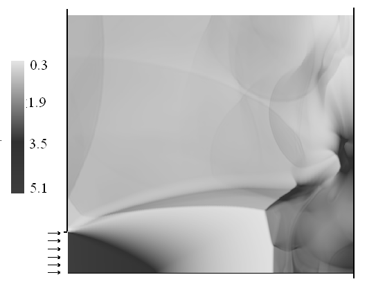Figure 2a. Supersonic jet impinging on the plane surface, the calculated flow

Figure 2b. Supersonic jet impinging on the plane surface, the inversed flow

Interactions of these elements may induce self-oscillations, according to the proposed mechanism of self-oscillations. First, there is the main shock formed as a result of jet braking before a plane (this shock is situated at right side of figure 2a). Further, the jet is limited by the contact discontinuity, which corresponds to the upper boundary of the dark shift, separating the jet from the outer media. Apart of it, there is the shock, going from the jet edge to it the central part, corresponding to the lower boundary of this shift. So, there are two intersection points of the main shock with mentioned above contact discontinuity and shock. Further, the main shock may be reflected from the symmetry axis as a Mach λ-configuration, to which break of the shock corresponds in figure 2a (this break is absent in some numerical variants). It should be added, that separation zone may appear between the main shock and the right solid surface in figure 2a. This separation zone was observed in some experiments[19] and appears in the part of numerical variants of this work, but is absent in the considered flow. At last, if to consider the jet with identical parameters, but flowing to the plane surface from right side to left one (corresponding flow is shown in figure 2b), and bring them closer to each other, then separating solid surface may be taken away, and both parts of the flow willl not change. Consequently, the number of “active” elements should be doubled.

So, this flows contains two or three intersection points and one or two contact discontinuities, and effect of perturbations reflection from the plane surface doubles these numbers. Thus, there is an ensemble of “active” elements and large number of possible interactions between these elements. It explains existence of unsteady regimes of considered flows, according to the proposed mechanism of self-oscillations. Disappearing of some these elements may explain decreasing of the oscillation amplitude and appearing of “silence” zones[19], but such effects require more detailed investigations.

To verify the numerical method described in the second section of this article a comparison of experimental and numerical values of main oscillation frequency is carried out. 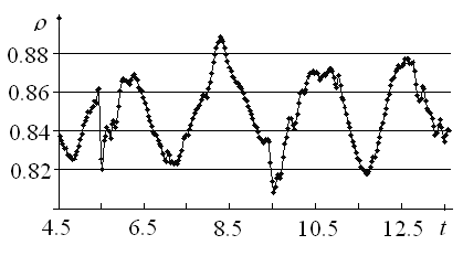The flow shown in figure 2a is defined by parameters =2.098 ( Mach number at the exit cross section of the nozzle), =4.785, γ=1.4 (specific heat ratio), h=6.95 (h – the distance between the nozzle exit and the right surface, - the nozzle radius), =4° (the nozzle half-angle). According to experimental data[20], this variant corresponds to a region with intensive self-oscillations, that is to say it is situated outside of "silence" zones. Frequency spectrum has spades, first of which is arranged at the frequency 9033Hz. To evaluate dynamics of the calculated flow the density history (figure 3) at brake point y=0 at the right plane may be used. It has 6 spades, noted by arrows. Middle distance T between these spades may be calculated as time distance between first and sixth spades (approximately 11.2), divided by 5 – number of intervals between spades. If to substitute the calculated thus dimensionless value T=2.24 to formulae ω=/(T) for frequency, if to use parameters =1.29kg/m³, =98066kg/(ms²) of the air under normal conditions and the nozzle radius =0.015m[20], the frequency value ω=8206Hz may be received. Comparison with the experimental value ω=9033Hz gives an evaluation of accuracy of numerical data. These data are received for the mesh with 696463 cells. The mesh with 546363 cells was used in [13] for the calculation of this flow and the frequency value ω=8041Hz was received

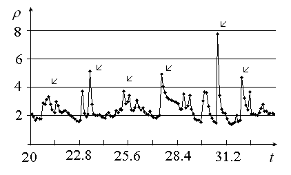Figure 3. Supersonic jet impinging on the plane, the density history at the brake point

4. Interactions of Inhomogeneous Streams with Blunted Bodies

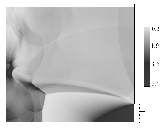
Search of flows with ‘active’ elements in the class of inhomogeneous flows near spherically blunted cones was started from the case supersonic stream + isobaric subsonic jet. This case does not provide large number of ‘active’ elements. Namely, the bold shock is transformed to the set of compression waves near boundary of the jet, and crosses this boundary without forming an intersection point. Some flows contain a tail shock, which crosses the jet boundary and produces intersection point. Another type of amplifiers is a contact discontinuity. One ‘active’ element of this type is available in the considered family of flows always, it is the jet boundary. Some flows contain circulation zones near surfaces of bodies. So, there are one or two contact discontinuities and one intersection point or absence of such points. This set of “active” elements is pure. Since surfaces of considered bodies are convex, the reflection of disturbances leads to their dispersing and does not support self-oscillations. So, significant self-oscillations, visible at the initial, but sufficiently large time interval[9-11], fade little by little, as a rule.

To find flows with intensive and stable self-oscillatory regimes an attempt to include the effect of disturbances reflection from solid walls is made. Namely, cone spherical blunts, dispersing disturbances, are replaced by more complicated blunts, containing plane and arched parts (figures 4a, 4b). The plane part is assigned to reflect disturbances without dispersing and to conduce to a generation of self-oscillations. But if to consider isobaric jets, self-oscillations are not large for both cases a) subsonic jet + supersonic stream and b) supersonic jet + subsonic stream. Cases subsonic jet + subsonic stream and supersonic jet + supersonic stream are not considered.

Next study is made for supersonic underexpanded jets. In this case additional points of the discontinuities intersection appear. As a result, self-oscillation amplitudes become large. Figures 4a and 4b show density distributions at different times for the unsteady flow, defined by parameters (the stream Mach number), =1.0323, (ratio of the jet radius and of the cone radius at the end of the blunt arched part), 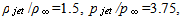the cone half-angle the employed mesh has 859725 cells.

Boundary conditions for the computation are no-flow on solid surfaces, prescribed variables on the inflow boundary, which is situated at left hand sides of figure 4a-4b, extrapolation on the outflow boundary. But if vortexes appear in the flow, the extrapolation condition leads to instability near outflow boundary when vortex approaches to it. In this case velocity component, normal to boundary, is prescribed to be non-negative at mesh points, nearest to this boundary. It allows to prevent instability and vortex reflection, but requires to exclude vicinity of this boundary from considering. The jet is running out from the cylindrical nozzle, situated at distance from the cone blunt.

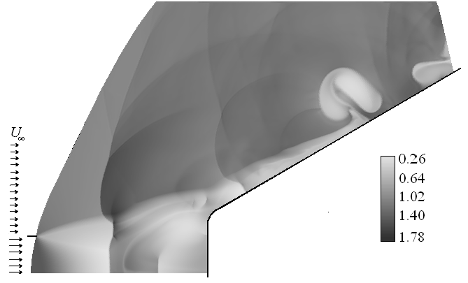Figure 4a. Density distribution near the blunted cone, the most distance of the bold shock from the blunt

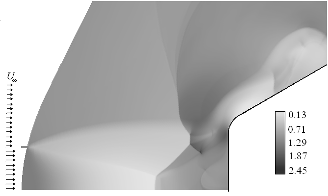Figure 4b. Density distribution near the blunted cone, the least distance of the bold shock from the blunt

Figures 4a and 4b show, that bold shock oscillates significantly, and intersection point of this shock and the jet edge oscillates with especially large amplitude (figure 4a shows nearly most left, 4b most right positions of this point). It can be seen in figure 4a, which shows the large part of the flow, that the layer near the cone surface has tendency to roll up.

This flow is calculated for grid numbers 640544 and 859725. Figure 5 shows the density history at the centre of the cone blunt for these grids. Satisfactory agreement of solutions may be seen.

Specific features of the oscillations visible in this figure are large amplitude and nearly periodic character. The last one may be explained, if to suppose that there is dominant resonance interaction, which defines oscillation period, and some interactions with small amplitudes. Another type of oscillations takes place, for example, in supersonic jet impinging on plane surface. In this case flow contains many ‘active’ elements and, perhaps, two or more interactions with amplitudes of the same order, which provides nearly stochastic type of self-oscillations (figure 3).

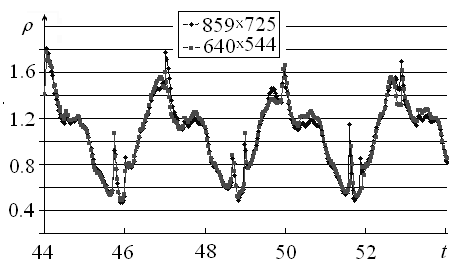Figure 5. The flow near the blunted cone, density histories for two meshs

To evaluate the effect of the disturbances reflection from plane blunt the last variant is calculated for the cone with the spherical blunt. As a result of blunt change the distance between the nozzle and the cone blunt changes too and becomes The density distribution for the new flow is shown in figure 6a and the density history at the brake point is shown in figure 6b. Significant decreasing (about 20 times) of the self-oscillation amplitude compared with the previous case (figure 5) may be seen. So, the dispersing effect turns off positive influence of reflected disturbances at producing of self-oscillations.

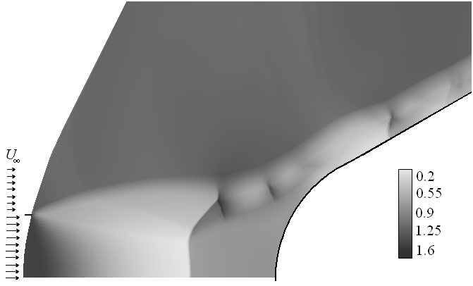Figure 6a. The density distribution near the spherically blunted cone

Figure 6b. The flow near the spherically blunted cone, the density history at the brake point

5. Conclusions

So, considered numerical data allow to suppose, that self-oscillations may appear as a result of resonance interactions of “active” elements - contact discontinuities and intersection points of shocks with shocks or shocks with contact discontinuities. Three theoretically possible types of interactions: 1 - contact discontinuity with contact discontinuity, 2 – intersection point with contact discontinuity and 3 - intersection point with intersection point - .are represented in considered flows, as a rule, in mixed form. The third type is represented both in classical self-oscillatory flows and in new unsteady inhomogeneous flows near blunted bodies. Since appearance of interaction of disturbances from intersection points and reflected from plane blunt disturbances in these flows induces strong growth of the self-oscillation intensity, it seems that self-oscillations of high amplitude are generated as a result of third type interactions. Considered data are not enough to evaluate exactly first and second interaction types, but it seems that these interactions may produce self-oscillations of relatively small amplitude.