1. Introduction

In the process of theoretical studies on the nature of these or those physical phenomena the problem of adequacy plays a vital role for the mathematical models that are designed to describe these phenomena. For example, if it is found that some physical phenomenon is actually realized in practice, then the one or other mathematical model will be adequate to it if and only if this model has the solutions that meet this phenomenon, and these solutions are stable[1-3].

Unfortunately, today the problem of the adequacy of mathematical modeling of physical phenomena has no satisfactory solution. Currently, for the selection of adequate mathematical models the approach that is based on a comparative analysis of experimental, analytical and numerical results is being used as a rule. However, we must admit, this approach is very time-consuming and, what is vital, still has not received adequate scientific justification. As for simple, effective and versatile analytical methods for selection of mathematical models, they have not been created yet.

In this paper we propose an analytical method of selecting adequate mathematical models of the hydrodynamic type. Its essence lies in the algorithmic construction of Lyapunov’s functionals[4, 5], which grow over time along the solutions of the corresponding initial boundary value problems for small perturbations. It allows you to establish results not only for theoretical (semi-infinite time intervals), but also for practical (finite time intervals) linear instability[6, 7]. It is important that it isn’t necessary to know the explicit form of the solutions to the problems for small perturbations.

The features of the proposed method are demonstrated below in the application to the classical problem of the linear stability of the steady-state spatial flows of an ideal incompressible fluid, which completely fills a vessel with rigid walls, in the absence of body forces to small three-dimensio- nal perturbations[1, 3, 8-13].

2. The Formulation of the Exact Problem

The spatial flows of an ideal incompressible fluid, completely filling a volume with a fixed solid impermeable boundary in the absence of body forces are being studied. These flows are described by the solutions of the mixed problem[2, 10, 13]

(1)

where – the velocity field, – the pressure field, – Cartesian coordinates, – time, – the normal to the surface – the initial velocity field of the fluid.

The stationary solutions of the initial boundary value problem (1) are also studied

(2)

and their absolute instability with respect to small three-dimensional perturbations and is being proved.

3. The Formulation of the Linearized Problem

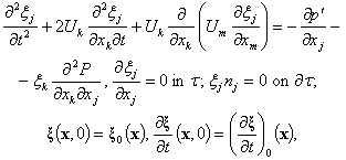
To achieve it the mixed problem (1) is linearized near the stationary solutions (2):

(3)

Here and – small perturbations of velocity and pressure fields, – the initial small perturbation of the fluid velocity field.

Unfortunately, the analogue for the integral of the kinetic energy to the initial boundary value problem (3) has not yet been found.

However, it can be constructed if the solutions of the mixed problem (3) are subject to special restriction – the condition of “equal-vorticity”[8, 12, 13]. The meaning of this provision is an integral form of the “freezing-in” condition of vortex lines in the field of virtual displacements of the fluid particles and it is expressed as the equality of velocity circulations along the contours obtained from each other with the volume preserving smooth mapping of the vessel with the fluid on itself.

“Equal-swirling” small spatial perturbations (3) can be described most clearly by the Lagrangian displacements field [14]:

(4)

In its turn, using equation (4) the initial boundary value problem (3) can be reformulated as follows

(5)

where – the initial Lagrangian displacements field, and – the initial first order partial derivative of the Lagrangian displacements field in time. Throughout the paper, for repeated indices of lower-case Latin letters the summing up from one to three is being carried out.

The analogue for the functional of the kinetic energy to the mixed problem (4), (5) serves as the integral[8]

(6)

Here – j-th component of a small perturbation of the vorticity field, – covariant pseudotensor of third order and the weight [15], – j-th component of the steady-state vorticity field.

Taking into account the expression (6) for the functional , we can conclude that among stationary solutions (2) of the initial boundary value problem (1) only those solutions that meet the rest states of studied fluid will be stable with respect to small spatial perturbations (4), (5) (and will be absolutely stable!).

In all other cases (including in the case of rigid-body rotation), the integral for small three-dimensional perturbations (4), (5) is neither sign-definite, no sign-constant, so the stationary solutions (2) of the mixed problem (1) corresponding to the steady-state spatial flows of considered fluid may be unstable with respect to these perturbations.

The following statement is just aimed at proving that there is the absolute instability in the linear approximation of the stationary solutions (2) which correspond to steady-state three-dimensional flows of the fluid under study.

4. The Lyapunov’s Functional

Next, an auxiliary integral[12, 13] is introduced into the consideration

(7)

The present functional is a volumetric integral over the vessel from the square distance between the fluid particles of perturbed (4), (5) and steady-state (2) flows of an ideal incompressible fluid in the phase space of solutions of the linearized initial boundary value problem (3).

As for the stationary solutions (2) of the mixed problem (1), without any generality limitations, the inequalities are true

(8)

where – known positive constant, then, through the differentiation of the functional (7) to the independent variable taking into account the correlations (4), (5), as well as using the expression (6) for the integral and the right part of the double inequality (8) it is easy to get a key ratio – basic differential inequality[13]

(9)

Here – some positive constant, throughout the article, the point above denotes the total time derivative.

As the procedure of integration of the relation (9) is described in detail in the work[16], the following results of the use of this procedure are reported only. That is, if a countable set of conditions is added to the differential inequality (9)

(10)

where a priori exponential lower estimate will be derived from this inequality with necessity

(11)

( – known positive constant).

It is worth noting that the class of solutions of the initial boundary value problem (4), (5) increasing with time according to the constructed estimate (11), with the additional conditions

(12)

on the initial data and is not empty.

In fact, since the mixed problem (4), (5) is linear, it is solvable with respect to small three-dimensional perturbations in the form of normal waves[1]. Further, since the functional (6) does not have the properties of sign-identification or sign-constancy, the initial boundary value problem (4), (5) is also solvable as related to increasing with time small spatial perturbations in the form of normal waves. Finally, any growing in time solution of the mixed problem (4), (5), which corresponds to a small three-dimen- sional perturbation in the form of a normal wave, due to arbitrariness of positive constant will satisfy the differential inequality (9), a countable set of conditions (10) and the lower estimate (11) identically and automatically. Consequently, the initial boundary value problem (4), (5), (12) has growing in time solutions that correspond to, at least, small spatial perturbations in the form of normal waves really that will be later illustrated by specific example.

Thus, the correlation (11) shows clearly that, as a minimum, one small three-dimensional perturbation (4), (5), (12) of the steady-state spatial flows (2) of an ideal incompressible fluid increases with time, at that not slower than exponentially. Since this ratio is found without applying requirements of restrictive nature to the steady-state three-dimensional flows (2), it implies the absolute instability of the latter with respect to small spatial perturbations (4), (5), (12).

In addition, the inequalities of relations system (10) are sufficient conditions for practical linear instability of steady- state three-dimensional flows (2) of an ideal incompressible fluid with respect to small spatial perturbations (4), (5), (12). As for small three-dimensional perturbations (4), (5), (12) in the form of normal waves, these inequalities are necessary and sufficient ones (in view of the fact that the positive constant is otherwise arbitrary). It is also important that these conditions for practical linear instability are inherently constructive. This property allows the use these conditions as the testing and control mechanism during physical experiments and numerical calculations.

In conclusion, it is appropriate to pay particular attention to the fact that the integral M (7) is the Lyapunov’s functional in this article, which grows over time in accordance with the motion equations of the mixed problem (4), (5), (12). A distinctive feature of this growth is a lot of freedom retained for the positive constant in the exponent index from the right side of the lower estimate (11). This freedom, in particular, allows us to interpret any solution of the initial boundary value problem (4), (5), (12), which increases with time according to the found priori exponential lower estimate (11), as an example of incorrectness according to Hadamard[17].

As it is demonstrated in the work[18] that the theory developed above can be extended on steady-state flows in unbounded closed areas, an illustrative analytical example of steady-state plane-parallel shear flows of an ideal incompressible fluid

(13)

where – a certain function of the independent variable in the space

between two quiescent rigid impermeable parallel planes ( – width of the gap) in the absence of body forces and superimposed on these flows small spatial perturbations in the form of normal waves

(14)

(here …, – some functions of its argument, – an arbitrary complex, and – some real constants), evolving in time in strict accordance with the constructed priori exponential lower estimate (11), is created further.

5. Example

Substituting expressions (13) and (14) into the motion equations of the mixed problem (4), (5) and the boundary condition

where – resting solid non-permeable parallel planes, which limit the infinite in length along axes channel – the fluid flow area studied here, an exception from the obtained relations of functions , and as well as the replacement of on a new unknown function lead to the classical boundary value problem of the eigenvalues and eigenfunctions detection for the Rayleigh equation[3, 9, 10, 19]:

(15)

In accordance with the results of papers[19-21], if the first relation of (15) is to be multiplied by the complex-conjugate function and then to separate in it real and imaginary parts from each other, it is rewritten in the form of an equivalent system of equalities:

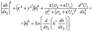(16)

Integration of correlations (16) on the cross-section of the interior layer between two non-moving solid impenetrable parallel planes applying boundary conditions (15) makes it possible, according to works[19-21], to come to the following equalities:

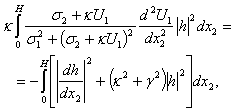(17)

From correlations (17), in agreement with the results of papers[19-21], it follows that exponentially growing solutions (14) () of the initial boundary value problem (4), (5) will be able to turn these correlations into identities if and only if the derivative changes the sign within the gap between two non-moving solid impenetrable parallel surfaces, and, at the same time, at least at one point of the latter the inequality holds true

(18)

However, for the quantity sign variation and the correlation (18), a completely different treatment can be suggested as compared with the ones that were proposed in the works[19-21].

In fact, if we carefully analyze the integral from the right side of the second equality (16), temporarily forgetting about the boundary conditions (15), it is easy to see that it can be written as

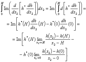(19)

It follows that the chain of correlations (19) will be equal to zero due to the boundary conditions (15), and only in those cases when

do not tend neither to 0/0, nor to

Unfortunately, the situation is possible when

and/or

because the function can consist of a countable set of branches. Examples of similar functions are logarithmic functions, inverse trigonometric and other functions.

It is impossible to choose one or another branch of the function ahead of time to find a solution to the problem (15). Surprisingly, but since into the formulation of the boundary value problem (15) there are not any conditions on the function (it is not involved in the formulation of the problem (15) at all!), there is no way to uniquely select one or another branch of the function for already found solution to the boundary value problem (15)! The present observation makes all branches of the function equal, that is, the integral (19) must vanish for all countable set of branches of the function as a whole that becomes a reason for the appearance of the type uncertainty.

From the above mentioned it follows that the solutions h of the problem (15) with functions consisting of a countable set of branches are not covered by the papers[19-21] results. These solutions will provide counterexamples to these results.

Thus, the results of works[19-21] are true not for all solutions h of the boundary value problem (15), but only for their particular class with functions consisting of a finite number of branches. Expanding the use of the papers[19-21] results is unjustified and wrong. This is confirmed by the specific example below.

Indeed, a subclass of steady-state flows (13) with the profile of the longitudinal velocity in the form[18]

(20)

where , and are arbitrary real constants, is considered further in this article.

With the help of the independent variable and the required function changes the ordinary differential equation (15), taking into account the correlation (20), can be shaped as follows

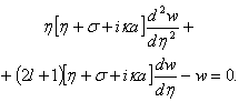(21)

If in the correlation (21) another change of the independent variable is to be carried out and take it is easy to make sure that it will be a variant of the Gauss hypergeometric equation[22]

(22)

The general solution of the correlation (22) is the function

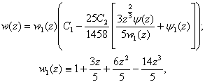(23)

(here and are some constants).

The boundary conditions (15) will hold for the function (23) if and only if

It follows that in this case the disperse correlation in the form

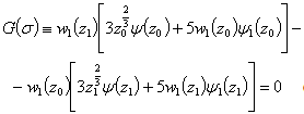(24)

must be satisfied. All appearing in the formula (24) functions of the complex variable are understood in the sense of its main branches.

Unfortunately, this disperse correlation cannot allow to calculate its roots through analytical methods, so one has to graphically explore the issue, whether it has roots that correspond to the exponentially growing small three- dimensio-nal disturbances in the form of normal waves (14), (15), or not (see Figures 1-3 below).

The essence of the graphic examination of the disperse correlation (24) to hold it roots, which correspond to the exponentially increasing small spatial perturbations in the form of normal waves (14), (15), is that first this correlation is rewritten in the form of Then, the curves (red lines in Figures 1-3) and (blue lines in Figures 1-3) are drawn on the complex plane . If as a result, these curves have the intersection points with the coordinates that it is these points will signal that the disperse correlation (24) has roots that correspond to the exponentially growing small three-dimensional disturbances in the form of normal waves (14), (15). Herewith, the coordinates of the intersection points of the studied curves and in numerical terms are being found using the coordinate grid through its suitable scaling.

The following are the results of the graphic dispersion correlation (24) study to hold it roots, which correspond to the exponentially growing small spatial perturbations in the form of normal waves (14), (15), for the three sets of characteristic parameters , and (see Figures 1-3 below, -axis is horizontal coordinate straight line, -axis – vertical one):

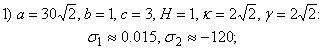(25)

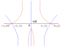Figure 1. Illustration to the data (25) (the origin is located at coordinates (0, -120))

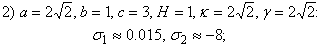(26)

Figure 2. Illustration to the data (26) (the origin is located at coordinates (0, -8))

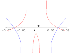
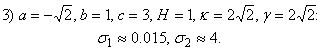(27)

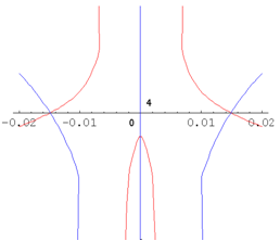Figure 3. Illustration to the data (27) (the origin is located at coordinates (0, 4))

It is important that these roots of the disperse correlation (24) do not coincide with any of the specific points of the functions of complex variable present in it.

Analyzing the data (25)-(27), first of all, it is necessary to note the fact that the velocity profiles (20), (25)-(27) of the steady-state plane-parallel shear flows (13) of an ideal incompressible fluid between two fixed hard waterproof parallel endless surfaces in the absence of mass forces have no points of inflection. Thus, the validity of the works[19, 21] results on the stability based on the immutability of the value sign for all three characteristic sets (25)-(27) of defining parameters can be observed.

As for the validity of inequality (18), for the velocity profile (20) with the parameters (25) it is true everywhere in the layer between the two non-mo- ving solid impenetrable parallel planes, for the velocity profile (20) with the parameters (26) – in the part of this layer, but for the velocity profile (20) with the parameters , (27) this inequality, on the contrary, is false anywhere within the gap between two non-moving solid impenetrable parallel unlimited surfaces. Hence, according to the results of articles[20, 21], at least, the steady-state plane-parallel shear flow (13), (20), (27) of an ideal incompressible fluid between two non-moving solid impermeable parallel planes in the absence of body forces must also be stable with respect to small spatial perturbations in the form of normal waves (14), (15).

However, the result (27) indicates clearly that, contrary to the results of works[19-21] on stability, the steady-state plane-parallel shear flow (13), (20), (27) of an ideal incompressible fluid within the layer between two non-moving solid impenetrable parallel infinite surfaces in the absence of body forces is still unstable with respect to small three-di- mensional perturbation in the form of normal wave (14), (15), (27).

Indeed, it is graphically found that the exponentially growing small spatial perturbation in the form of the normal wave (14), (15), (27) corresponds to the stationary velocity profile (20), (27). Of course, correlations (9), (11) as well as a countable set of conditions (10) are made for this perturbation.

Hence, it also follows that the action of the papers[19-21] results does not really apply to the small three-dimensional perturbation in the form of the normal wave (14), (15), (27). Therefore, the conditions for the linear stability[19-21] of the steady-state plane-parallel shear flow (13), (20), (27) can be satisfied for some small spatial disturbances in the form of normal waves (14), (15), but in no way for the small three-dimensional disturbance in the form of the normal wave (14), (15), (27). This testifies the necessary and sufficient nature of these stability conditions.

By the way, the function that appears in the general solution (23) contains a complex-valued inverse tangent and a natural logarithm (complex-valued too), so that its first-order derivative consists of a countable set of branches, and it is fully in agreement with the earlier reasoning.

As a result, the construction of an illustrative analytical example of the steady-state plane-parallel shear flows (13) of an ideal incompressible fluid within the limits of the gap between two non-moving solid impermeable parallel planes in the absence of body forces and imposed on these flows small spatial disturbances in the form of normal waves ( 14), developing over time in strict accordance with the designed a priori exponential lower estimate (11), regardless of whether linear stability conditions of the works[19-21] are true or not, has been completed.

6. Conclusions

In the present paper the problem of linear stability of steady-state three-dimensional flows (2) of an ideal incompressible fluid, which completely fills an arbitrary vessel with fixed solid impermeable walls, in the absence of body forces has been considered.

The direct Lyapunov method proves that the flows are absolutely unstable with respect to small spatial perturbations (4), (5), while the states of rest, on the contrary, are absolutely stable. We derive constructive sufficient conditions (see the inequalities of the system of correlations (10)) of the practical linear instability. A priori exponential lower estimate (11) has been constructed, which testifies to the time rise in the studied small perturbations. An illustrative analytical example of steady-state plane-parallel shear flows (13) of an ideal incompressible fluid between two non- moving solid impenetrable parallel unbounded surfaces in the absence of body forces and imposed to these flows small three-dimensional perturbations in the form of normal waves (14), that evolve over time in accordance with constructed a priori exponential lower estimate (11) regardless of whether the conditions of linear stability of works[19-21] are true or not, has been constructed.

It should be emphasized that from a mathematical point of view, the results of this paper are, for the most part, a priori, since the existence theorems for solutions to studied mixed problems for systems of differential equations with partial derivatives have not been proved.

Finally, concerning the question whether the mathematical model (1) adequately describes the physical property of liquids fluidity, it should be answered in the negative, because this model has no stable solutions (2), corresponding to the steady-state flows, although such flows are observed in nature and implemented in applications.

However, the current bad situation can be improved by the fact that if the conditions (see the inequalities of the correlations system (10)) of the practical linear instability are not carried out, stationary solutions (2) of the initial boundary value problem (1) are stable to the small spatial perturbations (4), (5), (12) in the form of normal waves at those or any other finite time intervals.

Thus, the mathematical model (1) does not adequately characterize the physical property of liquids fluidity in a theoretical sense (on semi-infinite time intervals), but adequately – in a practical one (on finite time intervals).

It follows that the constructive sufficient conditions (see inequalities of the correlations system (10)) of the practical linear instability may serve as a foundation for creation of an effective method for control of the steady-state flows (2) in real-time mode[23].

Indeed, suppose, for example, it is necessary to develop some technological process based on the use of steady-state flows (2).

In order for this process to be reliable in operation, it is necessary to ensure its practical stability for all admissible disturbances. In particular, the process must be stable in a practical sense with respect to the small three-dimensional perturbations (4), (5), (12) in the form of normal waves.

This goal can be achieved by constructing a numerical model that would meet the linearized mixed problem (4), (5), (12), with control at reference time points (10) for the validity of inequalities of the correlations system (10). During the construction of this model it is required to focus your major efforts on the fact that the inequalities of the correlations system (10) were not true at the expense of those or any other known external influences on the unsteady-state flows (4), (5) (for example, at the expense of the initial conditions (12) violation).

As a result, the practical stability of the developed technological process will be guaranteed, at least relative to small spatial perturbations (4), (5), (12) in the form of normal waves, and so the foundation will be laid for the creation of an effective method to control the steady-state flows (2) in real-time mode.

Unfortunately, the problem of constructing a numerical model described above (at least to date) has not been solved yet, and it is just waiting for the moment when experts pay their attention to it.

As there is no significant information about stationary solutions (2) of the initial boundary value problem (1) in the key differential inequality (9), it is justifiably to hope that this relation in either form will arise in the study of other mathematical models of hydrodynamic type. Therefore, the way of constructing Lyapunov’s functionals presented in this paper, which are characterized by a property to increase with time according to the interesting linearized equations of motion, will undoubtedly be a great help in ensuring the adequacy of the mathematical modeling of fluidity, at that not only for liquids, but also for other physical media (such as gases, plasma, and the like).

Finally, the present conditions of practical linear instability (see the inequalities of the correlations system (10)) can be interpreted as a numerical algorithm, which is built without digitization of appropriate defining differential equations for the first time in the history of science[24]. This fact indicates that with the aid of these conditions it is possible to set numerical results that in the degree of their accuracy, reliability and validity are in no way inferior to their corresponding analytical results. Thus, any distinction between numerical and analytical results is erased.

ACKNOWLEDGEMENTS

The author expresses his sincere gratitude and heartfelt thanks to A.M. Blokhin for the fruitful discussion of the results of this work and many pieces of good advice.

The study was supported by the Ministry of education and science of Russian Federation, project 14.B37.21.0355.