1. Introduction

Natural convection laminar flow of non-Newtonian power-law fluids from an isothermal horizontal circular cylinder plays an important role in numerous engineering applications those are related with pseudo-plastic fluids. The pseudo-plastic fluid is characterized by a constant viscosity at very low shear rates, a viscosity, which decreases with shear rate, at intermediate shear rates and an apparently constant viscosity at very high shear rates. The interest in heat transfer problems involving power-law non-Newtonian fluids has grown in the past half century. An excellent research on non-Newtonian fluids was performed by Boger[1]. Acrivos[2] was the first who considered boundary-layer flows for such non-Newtonian fluids. Since then, a large number of papers have been published, due to their wide relevance in pseudo-plastic fluids like chemicals, foods, polymers, molten plastics and petroleum production and various natural phenomena.

It should be noted that a complete survey of these literatures was impractical; however, selected papers are listed here to provide starting points for a broader literature search [3-15]. In the boundary-layer study, the previous researchers used the traditional power-law viscosity correlation that viscosity becomes infinite for small shear rates or vanishes for the limits of large shear rates, which are giving the unrealistic physical results. Because an infinite viscosity corresponds to solids and no frictionless fluid has ever been found, a partial set of measured viscosity shear relations are not sufficient for a boundary-layer study.

The recently proposed modified power-law correlation is sketched for various values of power index n, which has been shown in Fig. 2. The present model is formulated based on the available experimental data for the non-Newtonian fluids (see Boger[1]). It is clear that the new correlation does not contain the physically unrealistic limits of zero and infinite viscosity displayed by traditional power-law correlations[2]. The modified power-law, in fact, fits measured viscosity data well. The constants in the proposed model can be fixed with available measurements and are described in detail in Yao and Molla[16]. The boundary-layer formulation on a flat plate is described and numerically solved for non-Newtonian fluid in Yao and Molla[16, 17] and the associated heat transfer for two different heating conditions is reported in Molla and Yao[18, 19] for shear-thinning fluid. In this investigation, the behavior of both shear-thinning and shear-thickening fluids on the natural convection laminar flow from a uniformly heated horizontal circular cylinder are studied by choosing the power-law index as n (=0.6, 0.8, 1.0, 1.2, 1.4) to fully demonstrate the performance of various non-Newtonian fluids.

2. Formulation of the Problem

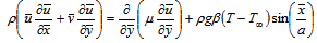
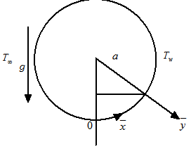
A steady two-dimensional laminar natural convection boundary-layer of a non-Newtonian fluid over an isothermal horizontal circular cylinder of radius ‘a’ with uniform surface temperature and a distributed heat source of the form has been considered. The viscosity depends on shear rate and is correlated by a modified power-law. We consider shear-thinning and shear-thickening situations of non-Newtonian fluids. 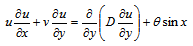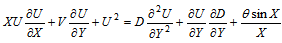It is assumed that the surface temperature of the cylinder is , where, is the ambient temperature of the fluid and T is the temperature of the fluid. The configuration considered is as shown in Fig. 1.

Under the above assumptions, the boundary-layer equations governing the flow and heat transfer are

(1)

(2)

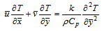(3)

Where and are velocity components along the and axes, is the fluid density, is the dynamic viscosity of the fluid in the boundary-layer region, g is the acceleration due to gravity, is the coefficient of thermal expansion, k is the thermal conductivity and C_p is the specific heat at constant pressure.

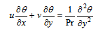
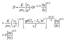
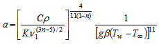
The kinematic viscosity is correlated by a modified power-law, which is

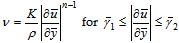(4)

The constants are threshold shear rates, which are given according to the model of Boger[1], K is the dimensional constant, for which dimension depends on the power-law index n. The values of these constants can be determined by matching with measurements. Outside of the preceding range, viscosity is assumed to be constant; its value can be fixed with data given in Fig. 2.

The boundary conditions for the present problems are

(5a)

(5b)

We introduce non-dimensional dependent and independent variables according to,

(6)

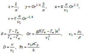
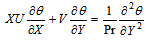
Where, is the reference viscosity at , is the non-dimensional temperature of the fluid, Gr is the Grashof number and Pr is the Prandtl number. Using equation (6) in equations (1-4) we get the following non-dimensional equations:

(7)

(8)

(9)

(10)

The length scale associated with the non-Newtonian power-law is

(11)

The corresponding boundary conditions are

(12a)

(12b)

Now we introduce the parabolic transformation:

(13)

Substituting variable (13) into equations (7)-(10) leads to the following equations:

(14)

(15)

(16)

(17)

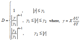
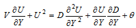
The correlation (17) is a modified power-law correlation first presented by Yao and Molla[16]. This correlation describes that if the shear rate lies between the threshold shear rates , then the non-Newtonian viscosity, D, varies with the power-law of γ. On the other hand, if the shear rate does not lie within this range, then the non-Newtonian viscosities are different constants, as shown in Fig. 2. This is a property of many measured viscosities.

Equation (14-16) can be solved by marching downstream with the leading edge condition satisfying the following differential equations, which are the limits of equations (14-16) as X→0.

(18)

(19)

(20)

The corresponding boundary conditions are

(21a)

(22b)

Equations (14-16) and (18-20) are discretized by a central-difference scheme for the diffusion term and a backward-difference scheme for the convection terms. Finally, we get an implicit tri-diagonal algebraic system of equations, which can be solved by a double-sweep technique. The normal velocity is directly solved from the continuity equation. The computation is started at X=0 and marches to downstream to X=3.1416. After several test runs, converged results are obtained by using ΔX=0.0025 and ΔY = 0.005.

In practical applications, the physical quantities of principle interest are the local skin-friction coefficients C_f and the local Nusselt number Nu, which are

(23)

(24)

Figure 1. The flow model and coordinate system

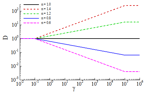Figure 2. Modified power-law correlation for the power-law index n (=0.6, 0.8, 1.0, 1.2, 1.4) while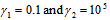

3. Results and Discussion

The numerical results are presented for the non-Newtonian power-law of shear-thinning fluids ( n = 0.6 and 0.8) and the shear-thickening fluids (n = 1.2 and 1.4) as well as the Newtonian case (n = 1) while the Prandtl number, Pr = 10 and 50. Based on the experimental data of Boger[1] the thresholds shears have been chosen as 0.1 and 10⁵, respectively. The obtained results include the viscosity, velocity and temperature distribution, velocity gradient and the wall shear stress in terms of the local skin-friction coefficient, and the rate of heat transfer as a form of the local Nusselt number, for the wide range of the power-law index n (=0.6, 0.8, 1.0, 1.2, 1.4).

Figs. 3a and 3b show the viscosity distribution, D as a function of Y at selected X (=1, 2, 3) locations for Pr =10 and 50, respectively and n = 0.6. From Fig.3a, it is found for Pr =10 that there is one region of variable viscosity at X =1 and 3, but there are two such regions at X =2; the primary region lies from Y ≈0.0 to 1.1 and the secondary variable viscosity region lies between Y ≈1.37 to 2.19. On the other hand, only one variable viscosity region was found in the case of Pr =50 in Fig. 3b. Again, Figs. 4(a)-(f) show the viscosity distribution, D as a function of Y at X = 1, 2, 3 respectively with n = 0.6, 0.8, 1.0, 1.2, 1.4 for Pr = 10 and 50. It is clearly seen in Fig. 4c that there are two viscosity distribution regions for n=0.6 at X =2 of Pr =10; all other viscosity distributions are in one region.

The velocity distribution as a function of Y at the selected locations (X =1, 2, 3) for the different power-law indices (n = 0.6, 0.8, 1.0, 1.2, 1.4) are presented in Figs. 5(a-c) for Pr =10 and 5(d-f) for Pr =50, respectively. Fig. 5 shows that for shear-thinning fluids (n=0.6 and 0.8), the velocity increases due to the decrease of viscosities at the downstream region; consequently, the boundary–layer is thinned. On the other hand, for shear-thickening fluids (n = 1.2 and 1.4), the velocity decreases slowly and the boundary-layer is thickened as the fluid becomes more viscous. We may conclude that for Pr =50, the fluid velocity is smaller than that for Pr =10 and the boundary-layer thickness is larger for Pr =50 than that for Pr =10.

The corresponding temperature distribution are plotted for Pr =10 and 50 in Figs. 6(a-c) and 6(d-f), respectively. For both of these Prandtl numbers, at the downstream region, in the case of shear-thinning fluids, the variation of temperature in the boundary-layer is smaller than that of the shear-thickening non-Newtonian fluids. As expected, the thermal boundary-layer is thinner for larger Prandtl numbers.

Figures 7(a-c) and 7(d-f) show the corresponding velocity gradient for Pr =10 and 50, respectively. For the shear-thinning fluids (n=0.6 and 0.8), the boundary-layer thickness decreases more at the downstream region than for the shear-thickening fluids (n = 1.2 and 1.4). The boundary-layer thickness for Pr =50 is almost half of the boundary-layer for Pr =10.

Figure 3. Viscosity distribution for different values of X at n = 0.6 for (a) Pr = 10, (b) Pr = 50

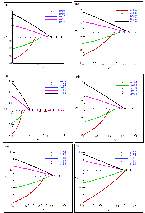Figure 4. Viscosity distribution for different n at (a) X = 1, Pr = 10, (b) X = 1, Pr = 50, (c) X = 2, Pr = 10, (d) X = 2, Pr = 50, (e) X = 3, Pr = 10, (f) X = 3, Pr = 50

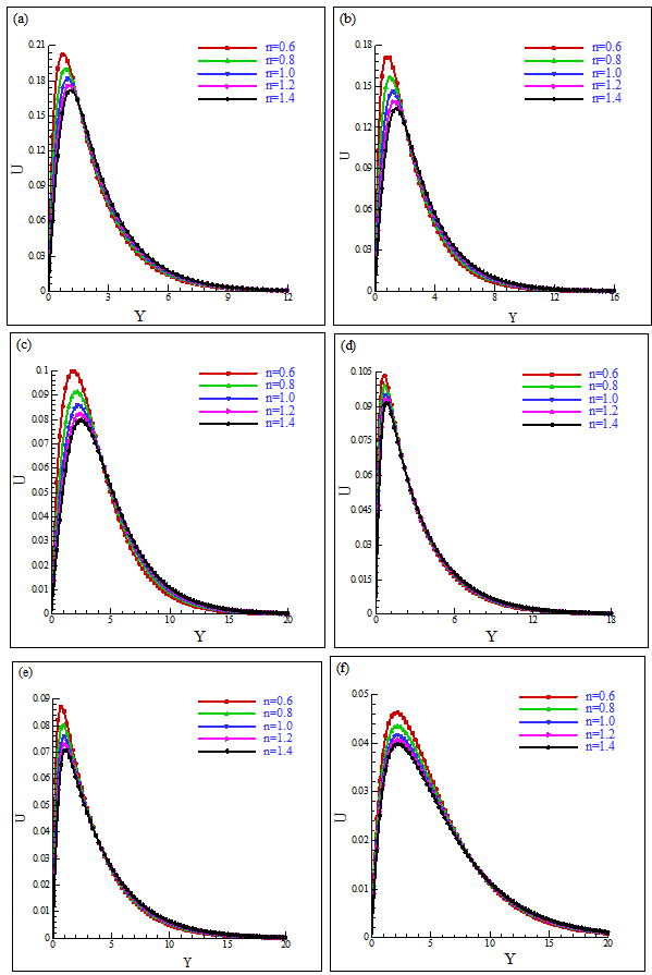Figure 5. Velocity distribution for different n at (a) X = 1, (b) X = 2, (c) X = 3; Pr = 10 and (d) X = 1, (e) X = 2, (f) X = 3; Pr = 50

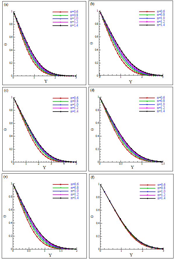Figure 6. Temperature distribution for different n at (a) X = 1, (b) X = 2, (c) X = 3; Pr = 10 and (d) X = 1, (e) X = 2, (f) X = 3; Pr = 50

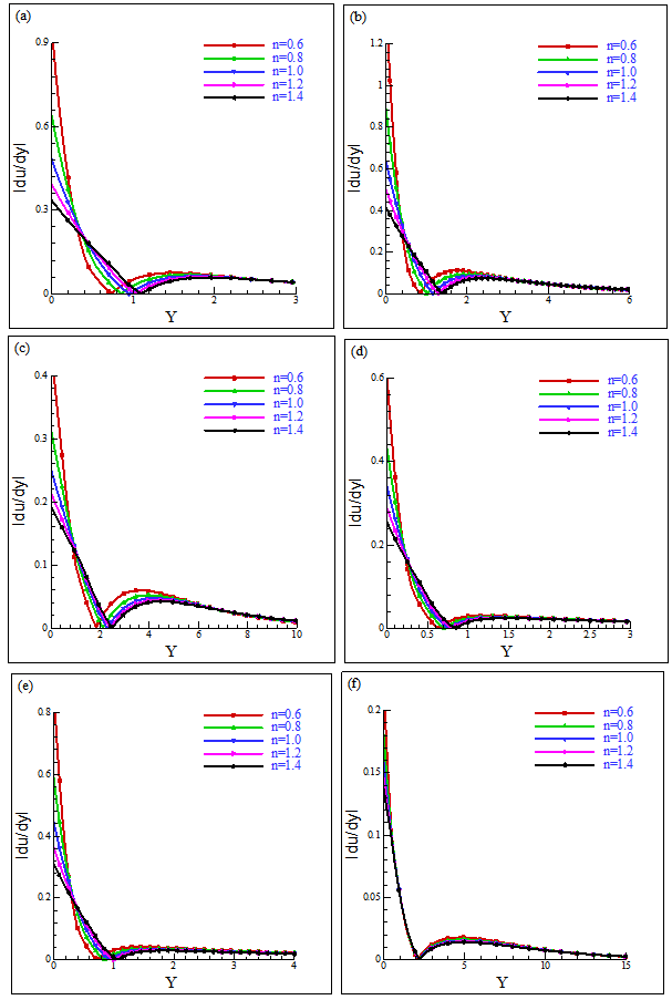Figure 7. Velocity gradient for different n at (a) X = 1, (b) X = 2, (c) X = 3; Pr = 10 and (d) X = 1, (e) X = 2, (f) X = 3; Pr = 50

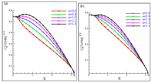
The effects of the non-Newtonian power-law index n (=0.6, 0.8, 1.0, 1.2, 1.4) on the variation of the wall shear stress are shown in Fig. 8a for Pr =10 and in Fig. 8b for Pr =50. The results from these figures clearly show that at the leading edge of non-Newtonian fluids, whose effects start from for Pr =10 and for Pr =50, the wall shear stress decreases for the shear-thinning fluids (n=0.6 and 0.8) and increases for the shear-thickening fluids (n=1.2 and 1.4). 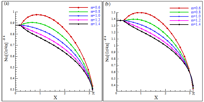At the downstream region, there is a similarity solution at and at , the boundary-layer of shear-thinning fluids is greater than that of shear-thickening fluids. As expected, the boundary-layer is thinner for larger Prandtl number. Figs. 9(a) and 9(b) represent the local-rate of heat transfer in terms of the local Nusselt number for Pr =10 and Pr =50, respectively. The local Nusselt number increases for n < 1 and decreases for n > 1 at the leading edge of non-Newtonian fluids, whose effects start from for Pr =10 and for Pr =50. At the downstream region, heat transfer is similar at .

Figure 8. Wall shear stress for different values of n: (a) Pr =10, (b) Pr = 50

Figure 9. Local Nusselt number for different values of n: (a) Pr =10, (b) Pr = 50

4. Conclusions

This study deals with the laminar two-dimensional natural convection boundary-layer flow of non-Newtonian fluids along an isothermal horizontal circular cylinder using a modified power-law viscosity model. The proposed modified power-law correlation agrees well with the actual measurements for non-Newtonian fluids; consequently, it is a physically realistic model. The problem associated with the non-removal singularity introduced by the traditional power-law correlations do not exists for the modified power-law correlation proposed in this paper. Therefore, we may conclude from the above numerical simulations that the proposed modified power-law correlations can be used to investigate other heat transfer related problems for shear-thinning or shear-thickening non-Newtonian fluids in boundary-layers. It is revealed that the effect of non-Newtonian fluids eventually becomes dominant when shear rate increases within the threshold shear limits. We may summarise our results from above simulations as follows:

●It is seen from the numerical simulations that the velocity increases due to the decrease of viscosities at the downstream region for shear-thinning fluids. However, the velocity decreases slowly as the fluid becomes more viscous for the case of shear-thickening fluids.

●At the downstream region of the boundary layer, the variation of the temperature inside the boundary-layer is smaller for the case of shear-thinning fluids than that of the shear-thickening non-Newtonian fluids for all Prandtl numbers considered here.

●The boundary-layer thickness decreases more at the downstream region for the shear-thinning fluids than that for the shear-thickening fluids. It is revealed that the boundary-layer thickness for Pr =50 is almost half of the boundary-layer for Pr =10.

●It is observed that the local Nusselt number increases when n < 1 and decreases when n > 1at the leading edge of non-Newtonian fluids for both Prandtl number considered here.

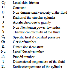
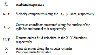
Nomenclature

Greek symbols

ACKNOWLEDGEMENTS

The second author wishes to thank Professor L. S. Yao, Arizona State University, USA, for the idea of the modified power-law viscosity model.