1. Introduction

Computer simulations are becoming a primary drive for the design and analysis of complex systems. The advancement of computing urges engineers to include high fidelity computational fluid dynamics (CFD) in the design and testing tools of new technological products and processes. Computational simulations are now recognized to be a part of the computer-aided engineering (CAE) spectrum of tools used extensively today in all industries, and its approach to modeling fluid flow phenomena allows equipment designers and technical analysts to have the power of a virtual wind tunnel on their desktop computer. Computational simulation software has evolved far beyond what Navier, Stokes or Da Vinci could ever have imagined. It has become an indispensable part of the aerodynamic and hydrodynamic design process for planes, trains, automobiles, rockets, ships, submarines, micro-electromechanical systems (MEMS), Lab-on-Chip (LOC) devices and so on; and indeed any moving craft or manufacturing process that mankind has devised so far. The advantage of numerical simulation with respect to experimentation is well-known.

Despite with these developments some primary issues of fluid dynamic simulations are like accuracy, computational efficiency and ability to handle complex geometries are predominant. A brief and concise literature survey on immersed boundary method, backward-facing step flows and the channel flows with obstructions are presented here. The governing equations and their numerical solution methods, including the boundary conditions employed are briefed in the next Section. The results and discussion are provided separately after that.

1.1. Immersed Boundary Method (IBM)

Fluids flows in complex geometries are very common in engineering problems, and the major difficulty arise in how to represent the body, its moving walls and its interaction with the fluid. The most usual approach is using Neumann and Dirichlet boundary conditions to represent the body geometry. Therefore, if the geometry is complex ones have a hard and, probably, a difficult work. This difficulty grows up if the body has a poignant and deformable geometry. In short, treating the coupling of the structure deformations and the fluid flow poses a number of challenging problems for numerical simulations. Both the unstructured grid method and IBM are used for simulating flow with complex geometries.

In most industrial applications, geometrical complexity is combined with moving boundaries and high Reynolds numbers which considerably increase the computational difficulties since they require, respectively, regeneration or deformation of the grid and turbulence modeling. As a result, engineering flow simulations have large computational overhead and low accuracy owing to a large number of operations per node and high storage requirements in combination with low-order dissipative spatial discretization. Given the finite memory and speed of computers, these simulations are very expensive and time consuming, with discretizations that are generally limited to a particular maximum number of nodes.

In addition to the above mentioned two methods, some authors have proposed different methods to treat this kind of problem. For example Harlow and Welch[1] proposed the marker and cell (MAC) approach. In this method the fluid region on one side of the boundary is identified by markers, while on the other side of the boundary, which can be fluid or solid, is identified by another marker. It requires huge storage space and CPU time.

In view of these difficulties it is clear that an alternative numerical procedure that can cope with the flow complexity but at the same time retain the accuracy and high efficiency of the simulations performed on fixed regular grids would represent a significant advance in the study of industrial flows. One possibility for the solution of this problem is the immersed boundary method (IBM).

The term “immersed boundary method” was first appeared in literature in reference to a method developed by Peskin[2] in the year 1972. A force term added to the Navier-Stokes equation is in charge to promote the interaction between fluid-solid interactions. Varieties of ideas have been proposed to calculate this force term leads to different immersed boundary techniques. Originally this method was used to simulate cardiac mechanics and associated blood flow. The distinguished feature of this method was that, the entire simulation was carried out on a Cartesian grid, which did not conform to the geometry of the heart. Hence, a novel procedure was simulated for imposing the effect of the immersed boundary (IB) on the flow. That is, imposing the boundary conditions is not straight forward in IBM. Since Peskin introduced this method, numerous modifications and refinements have been proposed and a number of variants of this approach now exist. The main advantages of the Immersed Boundary Method include computer memory and CPU time savings. Also easy grid generation is possible with IBM compared to the unstructured grid method. Even moving boundary problems can be handled using IBM without regenerating grids in time, unlike the structured grid method. It is to be noted that generating body conformal structured or unstructured grid is usually very cumbersome.

Imposition of boundary conditions on the IB is the key factor in developing an IB algorithm and distinguishes one IB method from another. In the former approach, which is termed as “continuous forcing approach”, the forcing function is incorporated into the continuous equations before discretization, where as in the latter approach, which can be termed the “discrete forcing approach”, the forcing function is introduced after the equations are discretized. An attractive feature of the continuous forcing approach is that it is formulated independent of the underlying spatial discretization. On the other hand, the discrete forcing approach very much depends on the discretization method. However, this allows direct control over the numerical accuracy, stability, and discrete conservation properties of the solver.

The merits of continuous forcing approach are its attractiveness for problems with elastic boundaries, closeness to the physics of the problem; hence relatively easy to conjure up the realistic flow problems especially high feasibility for successful simulation of biological and multiphase flows. The demerits of the aforementioned method include development of “stiff” numerical systems due to the presence of rigid Immersed Boundary in flow problems. Here satisfactory results have only been attained for low Reynolds number flows with moderate unsteadiness. Smoothing of the forcing function prohibits the sharp representation of the IB, which is not acceptable at high Reynolds numbers. The method also necessitates the computation in substantial amount of grid points located inside the body which simply results in unnecessary extra computation time.

The merits of discrete forcing approach include

(i) Suitability for flows around rigid bodies,

(ii) Handling of higher Reynolds number flows,

(iii) Absence of stiffness or user defined parameters that can impact the stability of the method,

(iv) The ability to represent sharp IB by imposing the boundary conditions directly on the numerical scheme and

(v) Computation of flow variables inside a rigid body becomes unnecessary.

Where as its demerits are need for a pressure boundary condition on the IB and moving boundaries are harder to deal with than in continuous forcing IBMs. A review about Immersed Boundary Methods (IBM) encompassing all variants is cited by Mittal and Iaccarino[3]. Feedback forcing method is applied to represent a solid body by Goldstein et al.[4] which induced spurious oscillations and restricted the computational time step associated with numerical stability.

Yusof[5] proposed a different approach to evaluate the momentum forcing function in a spectral method, and his method does not require a smaller computational time step, which is an important benefit of this method over preceding methods. The Discrete Immersed Boundary Finite Volume Method[6] used to simulate the present problem (i.e., to simulate the channel flows with obstructions) is based on a finite volume approach on a staggered mesh together with a fractional step method. The obstruction is treated as an Immersed Boundary. Both momentum forcing and mass source are applied on the body surface or inside the body to suit the no-slip boundary condition on the immersed boundary and also to satisfy the continuity for the cell containing the immersed boundary. In the IBM, the choice of an accurate interpolation scheme satisfying the no-slip condition on the IB is important.

The main advantages of the Immersed Boundary Method (IBM) include memory and CPU time savings. Also easy grid generation is possible with IBM compared to the unstructured grid method. Even moving boundary problems can be handled using IBM without regenerating grids in time, unlike the structured grid method.

1.2. Backward Facing Step Flows

The study of backward-facing step flows constitutes an important branch of fundamental fluid mechanics. Flow geometry of the same is very significant for investigating separated flows. This flow is of particular interest because it facilitates the study of the reattachment process by minimizing the effect of the separation process, while for other separating and reattaching flow geometries there may be a stronger interaction between the two. The principal flow features of the backward facing step flow are illustrated in Figure 1[7].

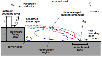Figure 1. Detailed flow features of the backward facing step flow

The phenomenon of flow separation is a problem of great importance for fundamental and industrial reasons. For instance it often corresponds to drastic losses in aerodynamic performances of airfoils or automotive vehicles. The backward-facing step is an extreme example of separated flows that occur in aerodynamic devices such as high-lift airfoils at large angles of attack. In these flows separation may be created by a strong adverse pressure gradient rather than a geometric perturbation, but the flow topology is similar. It is important in heat exchangers and gas turbines also. Since the location of the reattachment zone and its flow structure also determine the local heat and mass transport properties of the flow. This geometry has been received attention for half a century. Many researchers considered different aspects of this geometry from the flow pattern point of view and heat transfer. In some numerical simulations the backward facing step flow problem is a benchmark for validating the computational simulation algorithm.

The research in such a flow was escalated with the experimental and numerical work of Armaly et al.[8]. They presented a detailed experimental investigation in backward-facing step geometry for an expansion ratio (H/h) of 1.9423, an aspect ratio (W/h) of 35 and Reynolds numbers (Re_D) up to 8000. Here D=2h denotes the hydraulic diameter of the inlet channel with height h, H the channel height in the expanded region and W the channel width. When Reynolds number exceeds 400; it has been noticed that the flow appeared to be three-dimensional, a discrepancy in the primary recirculation length between the experimental results and the numerical predictions. Also a secondary recirculation zone was observed at the channel upper wall corresponding to higher Re values. Armaly et al.[8] conjectured that the discrepancy between the experimental measurements and the numerical prediction was due to the secondary recirculation zone that perturbed the two-dimensional character of the flow. The normalized value of the reattachment length showed a peak at Re_D =1,200. The decrease in recirculation length beyond a Reynolds number of 1,200 was attributed to the effect of Reynolds stresses.

Kim and Moin[9] numerically imitated the flow over a backward-facing step using a method that is second-order accurate in both space and time. Their results are (variation of the reattachment length on Reynolds number) in good agreement with the experimental data of Armaly et al.[8] up to about Re_D = 500. At Re_D = 600 the computed results of Kim and Moin[9] started to deviate from the experimental values. The discrepancy was due to the three-dimensionality of the experimental flow around a Reynolds number of 600.

By using a Galerkin based finite-element method, Gartling[10] developed a solution procedure for steady incompressible flow over a backward-facing step geometry. And the results are in good agreement with the results of Kim and Moin[9], especially with respect to the bottom wall separation zone. Lee and Mateescu[11] performed an experimental and numerical investigation of air flow over a two-dimensional backward facing step for Re_D < 3000. The hot film sensor measurements at Re_D = 5805 and expansion ratio H/h = 52.0 were found to be in agreement with their numerical predictions with respect to the locations of the separation and reattachment points on the upper and lower walls.

The bifurcation of two-dimensional laminar flow to three-dimensional flow was identified by Kaiktsis et al.[12]. This is the primary source of discrepancies appearing in comparisons of numerical predictions and experimental data. From their valuable work, it has also been observed that irrespective of the accuracy of the numerical schemes, the experimentally measured recirculation lengths were consistently underestimated above a Reynolds number value of Re_D =5600. They found that, all unsteady states of the flow are three-dimensional and develop for Reynolds number Re_D > Re_c (=700). Furthermore, they detected that the downstream flow region is excited through the upstream shear layer with a characteristic frequency f₁. The supercritical states (Re_D > 700) were found to be periodic with another incommensurate frequency, f₂ .

Numerical simulations of a symmetric sudden-expansion flow (2D) by Durst et al.[13] depicted the formation of secondary separation zones. This observation is similar to what is found in the backward-facing step flow. Both the experiments and the predictions confirm asymmetry-breaking bifurcation leading to one short and one long primary separation zone. Kaiktsis et al.[14] revisited the backward-facing step flow and found that the unsteadiness in step flow was created by convective instabilities. Another important conclusion of this study is that theupstream-generated small disturbances propagate downstream at exponentially amplified amplitude with a space-dependent speed in the range 700 < Re_D < 2500.

Heenan and Morrison[15] conducted experiments for a Reynolds number (Re_S) based on the step height S of 1.9x10⁵ and suggested that while the flow is likely to be convectively unstable over a large region, the global unsteadiness, driven by the impingement of large eddies at reattachment is the cause of low frequency oscillations called flapping. Erturk et al.[16] have presented a new, efficient and stable numerical method for the solution of stream function and vorticity equations. With this method they have presented steady solutions of driven cavity flow at very high Reynolds numbers (up to Re = 21,000) using very fine grid mesh. They have analysed the nature of the cavity flow at high Reynolds numbers.

2. Computational Methodology

To explain the concept of immersed boundary method, consider the simulation of flow past a solid body shown in Figure 2.

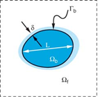Figure 2. Schematic showing a generic body past which flow is to be simulated

The body occupies the volume Ω_b with boundary Γb. The body has a characteristic length scale L, and a boundary layer of thickness δ develops over the body. In conventional approach, this would employ structured or unstructured grids that conform to the body. Generating these grids proceeds in two sequential steps. First, a surface grid covering the boundaries Γ_b is generated. This is then used as a boundary condition to generate grids in the volume Ω_f occupied by the fluid. If a finite-difference method is employed on a structured grid, then the differential form of the governing equations is transformed to a curvilinear coordinate system aligned with the grid lines[17]. Because the grid conforms to the surface of the body, the transformed equations can then be discretized in the computational domain with relative ease. If a finite-volume technique is employed, then the integral form of the governing equations is discretized and the geometrical information regarding the grid is incorporated directly into the discretization. If an unstructured grid is employed, then either a finite-volume or a finite-element methodology can be used. Both approaches incorporate the local cell geometry into the discretization and do not resort to grid transformations.

Now consider employing a non-body conformal Cartesian grid for this simulation, as shown in Figure 3. In this approach the immersed boundary (IB) would still be represented through some means such as a surface grid, but the Cartesian volume grid would be generated with no regard to this surface grid. Thus, the solid boundary would cut through this Cartesian volume grid. Because the grid does not conform to the solid boundary, incorporating the boundary conditions would require modifying the equations in the vicinity of the boundary. Precisely what these modifications are is the subject matter of IBM. However, assuming that such a procedure is available, the governing equations would then be discretized using a finite-difference, finite-volume, or a finite-element technique without resorting to coordinate transformation or complex discretization operators.

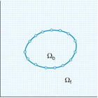Figure 3. Schematic of body immersed in a Cartesian grid on which the governing equations are discretized

2.1. Governing Equations

The general governing equations for unsteady, incompressible, viscous flow between parallel plates are written as

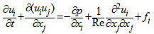(1)

(2)

where are the Cartesian coordinates, are the corresponding velocity components, p is the pressure, are the momentum forcing components defined at the cell faces on the immersed boundary or inside the body, and q is the mass source/sink defined at the cell center on the immersed boundary or inside the body. All the variables are non-dimensionalized by the bulk average velocity of the inlet flow, U_b and the length scales are non-dimensionalised by the channel height at the downstream, H. The only dimensionless number appearing in the governing equations is the Reynolds number.

For the flow problem considered, the following definition is used for the Reynolds number, Re.

(3)

Here and are the density and the dynamic viscosity, respectively

2.2. Geometry of Flow Domain and Boundary Conditions

Figure 4 depicts the two-dimensional channel with a backward facing step provided near the channel entrance. The finite distance in between the channel, which is small compared to its length and width makes the flow through this channel predominantly two dimensional. In addition, an incompressible Newtonian fluid with constant fluid properties is assumed as well. Buoyant forces involved are negligible compared with viscous and pressure forces.

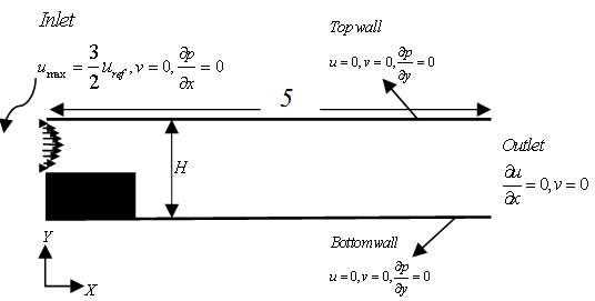Figure 4. Sketch of the flow configuration and definition of length scales

In order to simulate a fully developed laminar channel flow upstream of the step and to eliminate the corner effects, a standard parabolic velocity profile with a maximum velocity U_max=(3/2)U_b which is prescribed at the channel inlet for the present model. Cross stream velocity is equal to zero. The Neumann boundary condition can be assumed for pressure at the channel inlet. Fully developed velocity profile is assumed at the channel outlet. Pressure boundary condition need not be specified at the outlet No slip condition (u=0 and v=0) for velocity and Neumann boundary condition for pressure are considered corresponding to wall regions. The similar boundary conditions prevail when triangular obstructions are introduced in the channel.

To ease the comparison of the results obtained by the numerical simulation using IBM, the geometry of the backward facing step flow problem was chosen in accordance to the experimental setup of Armaly et al.[8]. The expansion ratio is defined by

(4)

That is, by the ratio of the channel height H downstream of the step to the channel height h of the inflow channel, where S denotes the step height. The results are generated for an expansion ratio of 1.9423. This expansion ratio was considered in the experimental study by Armaly et al.[8] and the same value has been used for a set of numerical computations with the Reynolds numbers values of 0.0001, 0.1, 1, 10, 50, and 100 by Biswas et al.[18]. The results have found to be agreeing quite well.

The time-integration method used to solve the above equations is based on a factional step method where a pseudo-pressure is used to correct the velocity field so that the continuity equation is satisfied at each computational time step. In this study, a second-order semi-implicit time advancement scheme (a third order Runge-Kutta method for the convection terms and a second order Crank-Nicholson method for the diffusion terms) is used. Eq. (1) and (2) are expanded as follows:

(5)

(6)

The velocity and pressure values are calculated using the following equations

(7)

(8)

(9)

(10)

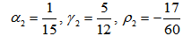
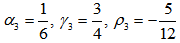
Where is the intermediate velocity, is the pseudo-pressure, is the computational time step, the sub-step index, and and are the coefficients of RK3 (Third order Runge-Kutta) whose values are

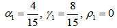(11)

(12)

(13)

A discrete-time momentum forcing function, should be appended with the Navier-Stokes equations to treat the immersed boundary (IB) as a kind of forcing so that it mimic the effect of IB. Here it is extracted from the literature presented Yusof[5]. This forcing function is incorporated to satisfy the no-slip condition on the immersed boundary (IB) and is applied only on the immersed boundary or inside the body. In the absence of IB, should be made equal to zero. The location of points, where the forcing function has to be introduced, is determined in a similar fashion as that of the velocity components defined on a staggered grid. When the forcing point coincides with the immersed boundary, momentum forcing is applied at that point so that the velocity is zero (see and in Figure 5). On the other hand, when the forcing point exists inside the body, momentum forcing is applied in such a way that the velocity ( or ) is the opposite of that ( or ) outside the body for both the wall-normal and tangential velocity components (respectively), as shown in Figure 5. However, because (no-slip) conditions and and come into the cell (as shown in Figure 6), the cell containing the immersed boundary does not satisfy the mass conservation. Hence, a mass source/sink termis introduced for the cell containing the immersed boundary to satisfy the mass conservation. The mass source/sink term is applied to the cell center on the immersed boundary or inside the body.

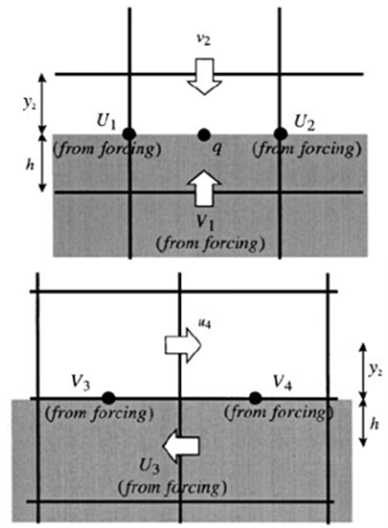Figure 5. Velocity vectors near the wall on a staggered mesh with wall-normal velocity and tangential velocity for a very simple situation (The shaded area denotes the IB)

2.3. Momentum Forcing and Interpolation for the Velocity

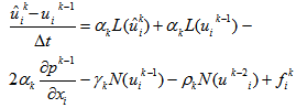
To obtain , from Eq. (5), the momentum forcing must be determined in advance such that satisfies the no-slip condition on the immersed boundary. When Eq. (1) is provisionally discretized explicitly in time (RK3 for the convection terms and forward Euler method for the diffusion terms) to derive the momentum forcing value, we have

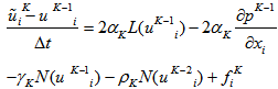(14)

Rearranging Eq. (14) results in the following equation for at a forcing point,

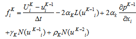(15)

Here is the velocity to be obtained at a forcing point by applying momentum forcing. In the following, in Eq. (5)) indicates the velocity at a grid point nearby the forcing point updated from Eq. (14) with to determine using the linear interpolation.

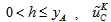
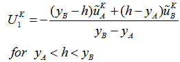
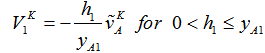
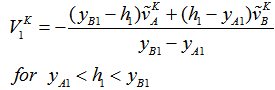
In case of the no-slip wall, is zero whenever the forcing point coincides with the immersed boundary. However, in general the forcing point exists not on the immersed boundary but inside the body, and thus an interpolation procedure for the velocity is required. In the present study, second-order linear interpolations are used, and Figure 6 shows the schematic diagrams for the calculation of interpolation velocity when the backward facing step is considered as the IB.

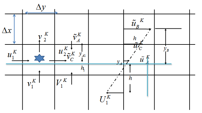Figure 6. Stencil for the linear interpolation scheme in the vicinity of backward facing step (IB) which shows instantaneous velocity, interpolation velocity, forcing points, etc

To explain the interpolation scheme distinctively with respect to Fig.6, the following second-order linear interpolation is considered

(16)

For is obtained from a linear interpolation between and the no-slip condition at the IB, whereas for 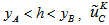is obtained from and . That is

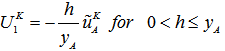(17)

(18)

The exact position of IB with respect to grids is determined and either Eq. (17) or Eq. (18) has to be used to calculate the U-interpolation velocity. The same scheme is applied to the y-component velocity. In the case of v-velocity, variant of Eq. (17) and Eq.(18) may be written as follows:

(19)

(20)

The exact position of IB with respect to grids is determined and either Eq. (19) or Eq. (20) has to be used to calculate the V-interpolation velocity.

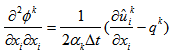
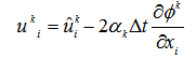
2.4. Mass Source and Continuity Equation

The procedure of obtaining the mass source in Eq. (6) is explained in this section. Consider the star marked two-dimensional cell shown in Fig. 6, where is the velocity components inside the body and, and are those outside the body. For the rectangular cell containing only fluid, the continuity reads

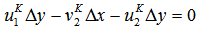(21)

Meanwhile, for the rectangular cell containing both the body and the fluid the continuity equation becomes

(22)

From Eq. (21) and Eq. (22), the mass source is obtained as . In general,

(23)

Note that is unknown until equations (6) and (7) are solved and thus we use instead of and is updated as and when is being found out. Therefore, in general the mass source is defined as

(24)

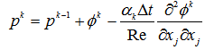
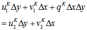
2.5. Solution Procedure

Figure 7. Flow chart for the Immersed Boundary Method

For the spatial discretization of Eq. (5) to (8) a finite volume approach on a staggered grid together with a fractional step method was employed. Being a CFD method, the Finite Volume Method (FVM) describes mass, momentum and energy conservation for solution of the set of differential equations considered. The FVM is comparable to other approximated numerical methods such as Finite Difference Method (FDM) and Finite Element Method (FEM). It is characterized by the partition of the spatial domain in a finite number of elementary volumes for which are applied the balances of mass, momentum and energy. The approximated equations for the method can be obtained by two approaches. The first consists in applying balances for the elementary volumes (finite volumes), and the second consists in the integration spatial-temporal of the conservation equations. In this work, the latter approach is followed.

The convection and diffusion terms were evaluated using a central differencing scheme of second-order accuracy. Solution of non-dimensional u and v are made possible in Alternating Direction Implicit (ADI) approximate factorization method clubbed with powerful and accurate Tri-Diagonal Matrix Algorithm (TDMA). The pressure solver is based on Successive Over Relaxation (SOR) method. The numerical code is developed using Digital Visual FORTRAN (DVF) and a detailed flow chart is shown in Figure 7, based on which the computer code is developed.

3. Results and Discussions

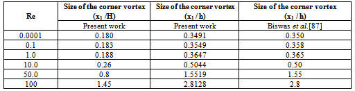
In order to ensure whether the predicted results are grid independent or not, extensive grid refinement studies were carried out. Finally, in backward facing step flow problem, the non -dimensional stream wise velocity at the centre of the channel outlet for Re=1.0 is tabulated (Table 1). It is seen that for the computational stencil of 252x102, percentage change of stream wise velocity with respect to previous stencil (202x82) is negligible. Hence the same grid size was selected for the code execution for all numerical examples presented here.

Table 1. Maximum non-dimensional stream wise velocity at the centre of the channel for different number of grids in horizontal and vertical directions at re=1.0 Maximum non-dimensional stream wise velocity at the channel exit Number of grids in stream wise direction Number of grids in cross stream direction 0.681687 27 7 0.763075 52 22 0.765939 102 42 0.766465 152 62 0.766649 202 82 0.766798 252 102

The general features of the two-dimensional flow field offered for an expansion ratio of H/h=1.9423 and a wide range of Reynolds numbers. This expansion ratio was considered in the experimental study by Armaly et al.[8]. It is found from the numerical computations that the flow over the backward-facing step is two dimensional and non-oscillatory in the region of Re_D < 100. This observation was well supported and commensurate with the experiments of Armaly et al.[8].

Figure 8 shows the stream wise velocity contours of the backward facing step flow problem in steady state flow field for an expansion ratio H/h=1.9423 for the Reynolds number range 10^-4 < Re < 10².

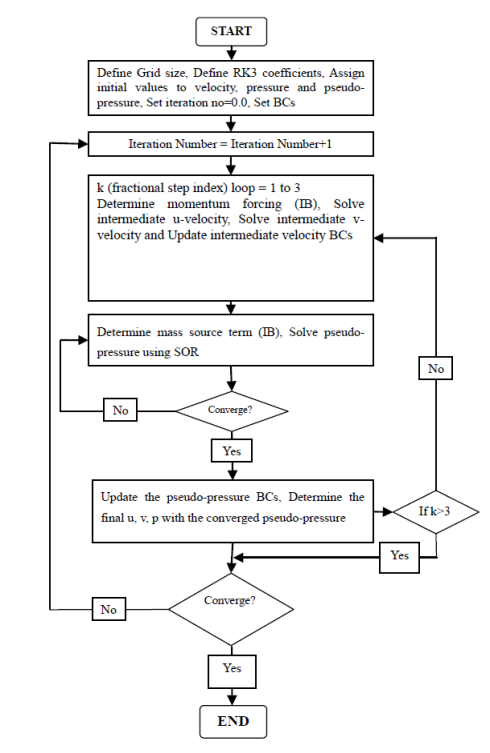
Figure 8. Stream wise velocity contours for backward facing step flow for different Reynolds numbers

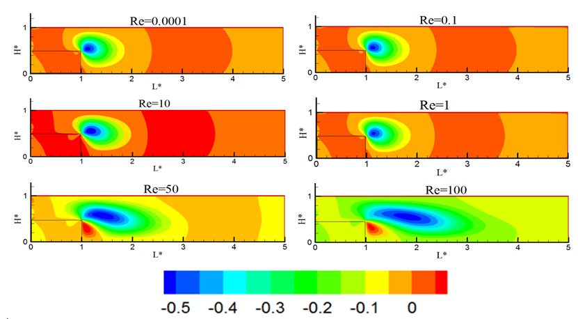Figure 9. Transverse velocity contours for backward facing step flow for different Reynolds numbers

Table 2. Comparison of the results for backward facing step flow

It is being observed that the maximum velocity is at the upstream side of the channel. A vortex is also visible at the concave corner behind the step. Stream wise velocity is being fully developed far downstream of the channel. It is being noted that immediately after the concave vortex, the fluid adjacent to the walls decelerates due to the formation of the two hydrodynamic boundary layers and backward pressure. Consequently, as a result of continuity principle, fluid outside these two boundary-layers accelerates. Due to this action, a transverse velocity component is engendered, which is clearly visible from the cross stream velocity contours generated for the aforesaid Reynolds numbers as shown in Figure 9, that sends the fluid away from the two plates outside the two boundary-layers and towards the centerline between the two walls. However, this action gradually decays with further increase in the axial distance downstream the backward facing step and finally vanishes when the flow becomes hydro dynamically fully developed.

It has also been observed that at low Reynolds numbers the flow separates at the sharp corner and then reattaches itself to the lower boundary further downstream forming a single primary re-circulating eddy. The reattachment length increases almost linearly with Reynolds number, the slight non-linear trend being attributed to viscous drag along the upper boundary. Computed non-dimensionalised reattachment lengths against inlet Reynolds number are shown in Table 2, to compare the same with the results of Biswas et al.[18].

Figure 10 shows streamlines of the steady state flow field for an expansion ratio H/h=1.9423 and a Reynolds number range 10^-4< Re< 10². It is evident from the stream lines that as the Reynolds number increases there is a backward flow occurring at the step, which is result of the negative pressure developed due to separation occurring at high velocity due to high Reynolds number. The plots well agree with literature especially commensurate with the experiments of Armaly et al.[8] which reveals that flow over the backward-facing step is purely two dimensional and non-oscillatory in the considered region. The streamline patterns for Re =10^-4, 10^-1, and 1.0 depict that the flow follows the upper convex corner without revealing a flow separation. Furthermore, a corner vortex is found in the concave corner behind the step. In this range of very small Reynolds numbers (10^-4< Re< 1), the size of this vortical structure is nearly constant varying between x₁/h=0.3491 (for Re=10^-4) and 0.3647 (for Re=1). Under these conditions, the effect of inertia forces can be assumed to be negligible compared with viscous forces often denoted as molecular transport. Hence the flow resembles the Stokes flow. Thus the determination of the separation and reattachment locations thus offers a severe bench-mark test for any hydrodynamic model because of the highly non-linear flow kinematics in the vicinity of the step.

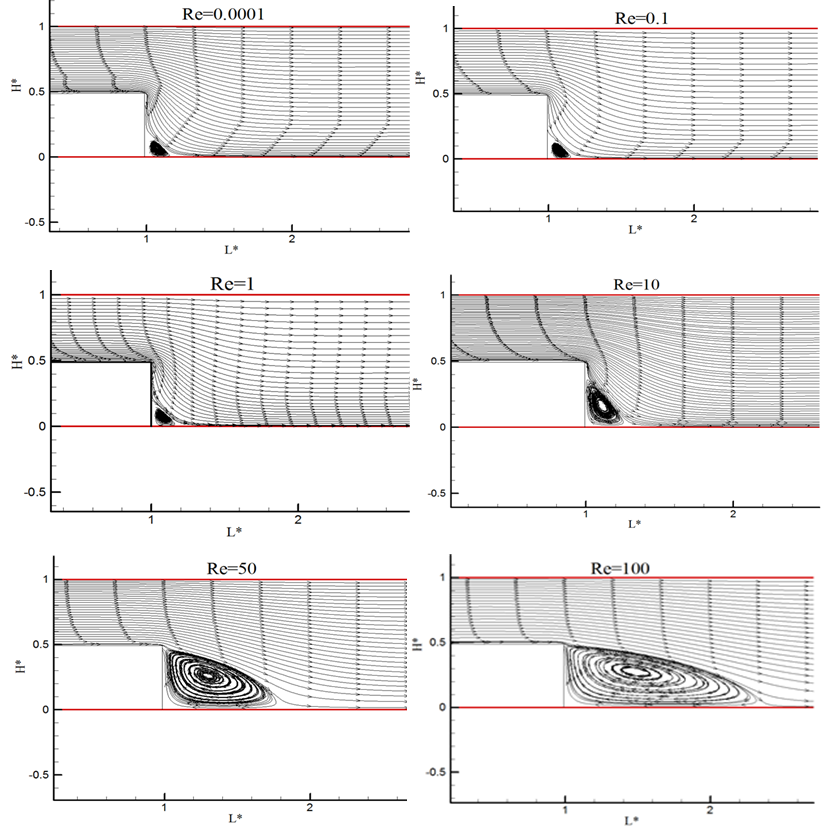Figure 10. Streamlines in the vicinity of backward facing step for different Reynolds numbers

Capturing of the corner eddies not only in backward facing step flow but also in flow with geometrical obstructions is numerically challenging and therefore, refined control volumes with the resolution in either direction of the flow domain is taken as Δx = 0.004 and Δy = 0.01. The entire domain was divided into 25704 control volumes and the code is run to generate the results with an accuracy of 10^-6 in all the cases. For the backward-facing step flow two important parameters are evidently responsible for the corner eddies. The first is given by the geometrical configuration, which can be defined by the expansion ratio H/h. The second is the Reynolds number. Fig. 10 clearly demonstrates the effect of the Reynolds number for a fixed expansion ratio H/h = 1.9423. The size of the corner eddy is nearly constant for all Reynolds numbers below Re_D = 1.0. However, for Re_D > 1.0 the corner vortex strongly increases in size. As a direct consequence, the corner vortex reaches up to the corner of the step at Re_D = 10.0 and covers the complete face of the step. Hence a change in the entire flow structure is observed and the notation of a corner vortex has to be replaced by the notation recirculation region, which for Re_D > 10.0 better reflects the flow structure. With increasing Reynolds number the size of the recirculation region steadily increases.

4. Conclusions

Immersed-boundary method is adopted to validate a relevant fluid mechanics bench mark problem, the backward facing step flow problem. The present method is based on a finite volume approach on a staggered mesh together with a fractional-step method. The momentum forcing and the mass source/sink are applied on the body surface or inside the body to satisfy the no-slip boundary condition on the immersed boundary and the continuity for the cell containing the immersed boundary, respectively. A linear interpolation scheme is used to satisfy the no-slip velocity on the immersed boundary, which is numerically stable regardless of the relative position between the grid and the immersed boundary.

The present algorithm is ideally suited to low Reynolds number flows also. Predictions from the numerical model have been compared against experimental data of different Reynolds numbers of flow past backward-facing step geometries. In addition, computed reattachment and separation lengths have been compared against alternative numerical predictions in the published literatures. Also, the immersed boundary method with both the momentum forcing and mass source/sink is found to gives realistic velocity profiles and recirculation eddies for the backward facing step flow problem demonstrating the accuracy of the method. By conducting this numerical study, we can conclude that immersed boundary method is a robust way of determining flow field and can rival experimental and laboratory study. Generally for backward facing step flow, the velocities are very small in the recirculation zone compared to the velocity of the mean flow. Hence the separation surface is submitted to a strong shear. In order to characterize the topology of the separated zone, measurements of the reattachment length in the stream wise direction may be captured.

The range of Reynolds numbers, where the analysis is made possible only in three dimensional way, may be identified by rigorous numerical experimentation. The discrepancy in the primary recirculation length between the experimental results and the numerical predictions in both 2D and 3D analysis may analysed critically. According to Armaly et alI[8], during experimentation a secondary recirculation zone was observed at the channel upper wall when the Reynolds number is greater than 400. It may also be ensured numerically that the discrepancy between the experimental measurements and the numerical prediction is due to the secondary recirculation zone that perturbed the two-dimensional character of the flow. Further numerical experimentation of poignant bodies may l\also be carried out.

ACKNOWLEDGEMENTS

This work was supported by the National Institute of Technology, Calicut, India.