1. Introduction

This paper is devoted to the problem of sound scattering by small chaotically situated spherically symmetric gas dynamic structures intended to model turbulent velocity fluctuations. If these structures were at rest then scattered field frequency spectrum will be the same as for each structure, while total scattered power will be the power scattered by any isolated structure multiplied by their number due to their chaotic space distribution[16]. A lot of experimental and theoretical works are devoted to chaotic motion media and to sound scattering[1-36]. For instance, in[14] Brown motion basic properties investigated in the beginning of previous century by A. Einstein and M. Smolukhovtsky are discussed as specific example of suspended particles chaotic motion. Brown motion laws are based on the following principle – particle displacements in any direction are equally probable, while inertial forces could be neglected with respect to friction forces influence governing particle motion. In[31] laws of Brown particles sound scattering are investigated in relation to low frequency sound scattered in their suspensions (solutions). However in this paper we shall be interested in opposite microinhomogeneous media example – the media where in particles (microstructures) motion viscose forces could be neglected with respect to corresponding inertial forces [35-36]. This is the case of developed (full-blown) turbulence and sound scattering there. Multiple works were devoted to this problem study[1, 3-6 and 8-22]. All of them are based on turbulent flows gas dynamic structure analysis as well as on definite microinhomogeneous media structure models. Possible turbulent media models could be separated in two classes – wave and corpuscular models. First type models are more widely spread. Most part of turbulent flows structure heuristic theories are based on wave model fundaments[1, 4, 6, 14-22 and 35-36].

Corpuscular models[2, 6 and 8-13] allow solving a sequence of application problems of flow and heat exchange description in wall layer turbulence[12], contributing as well to turbulent theory development[8]. One of the initial turbulence models developed by L. Prandtl was corpuscular[2]. Recent years give rise to specific part of turbulence theory related to study of “large” vortices role in mass and heat exchange processes. It is based on “coherent” turbulence model generated in turbulent jets, in wakes behind streamlined bodies, in preseparation regions of wall turbulent boundary layers and in nature (tornados, hurricanes) as well. Basis of turbulence model in[12] is a statement that vortices - structures of scale larger than molecules take major part in turbulent flow formation. In turbulent flow to be generated their behavior and sizes distribution obey specific laws allowing stochastic consideration. Traditional method of turbulence theory composition[8, 35-36] is based on Reynolds equation system. Basic equations and generalized kinetic theory relationships are formulated there to close up Reynolds equations system. It is shown that state of media in locally kinetic gas theory dynamics is defined by distribution functions sequence - not isolate distribution function. Each molecule group dynamic state function is derived from related Reynolds equations system. So, that after pooled data definition dynamic state of system is expressed by simple summation. We shall use same principle in total sound scattering definition.

Experiments on light scattering in turbulent and laminar flows[9-11] are most conclusive proof of turbulent media structure corpuscularity. It is well known that for turbulent fluctuations of definite substantion closed description in local point of flow two independent functions are customary used. Distribution function of substantion quantity fluctuations (say, velocity, temperature or touch concentration) acts as process amplitude characteristic. Fluctuations spectrum represents distribution of fluctuation energy over frequency range, characterizing process scale properties. Definite body of mathematics is developing or already developed for both characteristics[2-7, 12 and 13]. But such turbulent fluctuation description method suffers from few disadvantages. One of them lie in the fact that fluctuation spectrum is a process mathematization (harmonic analysis) product not describing fluctuation physical structure univocally[9-11]. Technical applications and a sequence of theoretical models require namely physically existing fluctuation scale knowledge. Moreover, it is difficult to acquire such important turbulence feature as intermittency with aid of distribution function. In experiments touch concentration changes being used to fluctuation optical perceptibility improvement were frequently of purely turbulent nature not complicated by additional factors such as molecular diffusion. That is why splinter process to be observed was close to splinter process predicted in[13], where logarithmically normal fractions dimensions distribution law was derived. In experiments existing scales of turbulent inhomogeneities (vortices) acquire mathematical definition together with such characteristics as “mole dimension” and few other widely used in physical phenomena corpuscular models (say, in combustion theory) called forth by turbulent mixing. As a whole these data are to be considered as turbulence corpuscular properties reflection and opposite to the spectrum governed by its wave properties. We shall try to develop similar approach to one of basic turbulent media physical properties – to sound scattering by full-blown turbulence description. Namely, not ignoring “wave model” progress and results, we shall try to develop turbulent medium scattering sound corpuscular model, based on the fact that this microinhomogeneous medium consists of multiple spherically symmetric chaotically moving gas dynamic structures – localized flows, say, vortices. In addition to variation of velocities and dimensions specifics of such structures, to be compared with results of[23-27], lies in the fact that media flow will be observed not only outside but inside such structures (inhomogeneity) as well. Each structure inside will consist not of rigid matter as in[23-25, 27], but of environment medium substance, say, of fluid (gas) as in[26]. In our model substance exchange between inner and outer structure regions will be allowed in principle. As before in[28-32], we shall consider the case of microinhomogeneous media – as media comprising great many microstructures (fluctuations or vortice) situated at distances smaller then incident sound wavelength. However, minimum distance between them should still substantially exceed structure linear dimension. If such identical structures were distributed uniformly over the entire volume, say in the form of regular lattice, then no scattering would be observed at all[16]. So that immediate case of scattering to be studied is chaotic structures distribution with their concentration being constant on the average only. Basis of low frequency sound scattering in such media lies in scattering law of single inhomogeneity (structure) of dimension small with respect to sound wavelength. For structures (particles) at rest classical Rayleigh law is valid[3, 16]:

(1)

in accordance to which, scattering crossection of sound is proportional to structure crossection multiplied by highly small quantity. Inhomogeneity concentration n and unit scattering crossection, determining media unite volume scattering capability, provide microinhomogeneous media wave attenuation property. Then sound intensity will decrease exponentially () with distance due to scattering on inhomogeneities. Logarithmic intensity attenuation γ, measured in dB per unit distance of sound wave travel takes the form. Formulating inhomogeneity volume and total inhomogeneity material unit content in medium τ through inhomogenety average radius and concentration (), we obtain γ in the form. In general, inhomogeneity scattering crossection [28-32], say, for moving inhomogeneity, could be expressed as a product of its crossection and some dimensionless function : , where - Mach number, - Reynolds number. Then we can write. In the presence of several ( types) types of particles (inhomogeneities) mixture, characterized by concentration n_i and unit scattering crossection, wave intensity will decrease exponentially with distance in accordance to law:

(2)

while logarithmic attenuation factor γ acquires the form:

.

For -th type of scatterer with radius a_i and concentration n_i, expressed through unit volume fraction τ_i (), total attenuation γ looks like:

.

Or taking into account expression for introduced above [32] , for total attenuation factor (decrement) we obtain:

(3)

For continuous scatterer size, concentration or velocities distribution last expression could be easily generalized in the integral form[31]. For turbulent media corpuscular model expression (3) is close in ideology to concepts of mentioned above paper[8], where dynamic state of media is determined by sequence of vortex system distribution functions each of which characterizes dynamic state of corresponding localized flow group. So that after determination of each function media state is provided by simple summation.

Most of microinhomogeneous media elements are moving [28-32]. It was shown for various types of scatterers[23-27], that corrections to sound scattering amplitude are proportional to hydrodynamic Mach number of their motion first degree and unlike light scattering is quite noticeable. Their motion influence is not only of kinematic but of dynamic nature as well and it could not be reduced to Doppler effect only. For the type of scattering to be studied wave scattering source is the same as in[28-32], namely chaotic scatterer positions or their chaotic motion.

Returning to turbulence sound scattering problem current state we should note, that its existing concept is by and large semi empiric[1, 4, and 15]. In other words, in expressions for scattered sound parameters derived on the basis of turbulent fluctuations heuristic spectra correction factors are to be frequently introduced. However sometimes, due to scattering theory contradictions, these minor corrections are insufficient. For instance, attenuation factor low frequency dependence ()[1] is not supported by experimental data. In the same time, development of adequate sound scattering theory for isotropic homogeneous turbulent media is possible on the basis of its behavior fundamental laws further study only.

2. Turbulence Corpuscular Model

From theoretical point of view the case of homogeneous isotropic turbulence is the simplest. But practically this case occurs rarely in turbulent flows. These conditions are violated for instance due to flow boundaries or to anisotropy introduced by space dependent mean velocity of turbulent flow. From the other hand, there are reasons to believe that large Reynolds number small-scale flow fluctuations in limited space regions will be locally homogeneous and isotropic. This hope is based on qualitative picture of full-blown turbulence origin proposed in last century 20-th by Richardson and developed by A.N. Kolmogorov and A.M. Obukhov[1-3, 6, 13, 35 and 36]. L.G. Loitsiansky fairly called turbulent flow velocity fluctuations as various scale vortices driving turbulent flow[6]. It is important to note, that viscosity plays no perceptible role in flow formation, for each scale Reynolds numbers are too large, and nonlinear effects govern this process first of all. That is why energy is not lost in the process of transfer from larger flow scales down to smaller scales. It is defined by scale independent quantity - energy per unit mass in that flow. Its value order was defined by dimensionality considerations as initial flow energy decrease[13, 18, 35 and 36]. The only value of dimension, to be constructed using and, is

(4)

Larger fluctuations to smaller splinter process goes on until viscosity forces take effect, i.e. up to scales (), for which (or, more precisely, ). These scales flow is hydrodynamically stable and not splinting further in smaller scales. Energy received by these scales in unit time is transferred directly to heat due to viscose forces. So that parameter defines energy dissipation of flow unit mass per unit time as well. In outer scale splinter to scale fluctuations – they are observed not only in direction of mean flow velocity. In other words, motion in scale is more isotropic then outer (average) flow. Similarly in scale generated by scale fluctuations isotropy will increase, while average flow influence – decrease and so on. As a result after few multiplication stages turbulent flow becomes isotropic. In other words, in full-blown turbulence most fluctuation scales, with exception of few largest, become statistically homogeneous and isotropic. Scale is called outer scale, while inner (Kolmogorov) scale[6, 13, 18 and 35, 36].

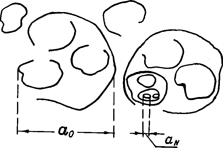Figure 1. Corpuscular model of full-blown turbulent medium. All possible sequential decreasing scales of contributing structures (fluctuations or vortices) from outer to inner (Kolmogorov’s) scale are presented[18]

The larger initial flow Reynolds number, the more its splinter stages with serially decreasing scales from until. That is why, for large initial Reynolds numbers, there exists representative scales “inertial” interval (), where, or, simply speaking, turbulence inertial interval. Qualitative picture of turbulence corpuscular model is shown on Fig.1.

All scales (dimensions) of vortices with sequentially decreasing scales from until inner Kolmogorov’s scale are presented in corpuscular turbulence structure. These fluctuations (vortices) being universal for any turbulent flow, they have forgotten about outer turbulent flow structure, while viscosity forces are still not important for their behavior. That is why this interval is characterized by two parameters - scale and energy flow velocity only. Few flow estimates to be used in the sections to follow could be derived easily on the basis of dimensionality considerations. Let us define first the order of fluctuation velocity for scale. It can depend on and, while the only possible combination of velocity dimension to be arranged using them be

(5)

With aid of (4), we can write

(6)

Reynolds number for arbitrary turbulence scale is

(7)

where - Reynolds number of initial (outer) flow. If we suppose that our estimates are fair until inner turbulence scale, for which, then the order of value of and corresponding fluctuation velocity are

(8)

So that and are decreasing with initial flow Reynolds number increase proportionate to and to respectively. From the point of sound scattering discussed below its worth to note, that relationship between and , defining scattering conditions for moving vortex[26-27 and 29] is reduced for large Reynolds numbers to relationship between sound frequency and ratio value, expressed in the form in accordance to (6).

3. Scattering Theory Contradictions

As to most important experimental data, it is widely believed that sound audibility decreases drastically in the presence of wind. This effect is observed on not very large distances and usually could not be explained by sound ray distortion in gradient wind flow[1]. It is directly related to wind turbulence. Dahl and Dewick were the first to point this effect out in 1937 in relation to fading observation[1, 34]. Sukharevsky confirmed a little later in 1940 it in Caucasus measurements. Bad sound audibility in wind condition was underlined by Stewart in 1919[1].

But most thorough experimental study was undertaken by Sieg in 1940[1, 33]. Не called attention to additional attenuation of sound in the presence of wind, attenuation substantially exceeding sound absorption related to air molecular properties (viscosity, heat conduction and air humidity - Knezer effect). Sieg basic results could be reduced to following. In the frequency range 250 - 4000 Hz in weak wind (1 - 2 m/s or in almost dead calm) perceptible intensity sound fluctuations (fading) are not observed, but intensity decreases with distance. But for all that even if molecular absorption will be subtracted, sound attenuation factor (decrement) comprises still up to 1,5 - 2,2 dB at 100 m. In Siegs experiments frequency dependence of was not detected. However, as to Siegs critics opinion, his observations accuracy was not substantial, sound source directivity was not taken into account and conditions of various frequency sound attenuation observations were not identical enough. So that his results may represent order of value estimate only, being approximately constant in the frequency range 250 - 4000 Hz. In strong gusty wind attenuation factor increases running up to 5 - 9 dB value at 100 meters (at gusty wind from 7 to 17 m/s). In these conditions frequency dependence of becomes observable, namely equals 5 dB for 250 Hz, 8 dB for 2000 Hz, 9 dB for 4000 Hz (at 100 meters). At the same conditions intensity fluctuations (fading) runs up to 25 dB. Effect explanation first attempts are related to first half of ХХ century. Turbulent flow influence on sound wave could be reduced to sound scattering resembling partly scattering of light traveling in turbid media: both cases comprises random fluctuations of propagation velocities. It is not out of place to note, that as it is shown in[28, 32], perfect analogy is not observed. Theoretical problem study in[1] proceeded from the version of moving media sound propagation wave equation – Obukhov equation approximately taking into account presence of vorticity in the medium. However, any conclusions related to specific role of vorticity in sound scattering was not done there. Farther, just like in[23-32] for Lighthill equation, to calculate scattering amplitude and attenuation factor sound scattering problem was solved in[1]. Scattered wave amplitude was shown to be

(9)

Factor was expressed through scattering amplitude and after integration and averaging it was derived in[1]

(10)

where, and - numerical factors related to turbulent fluctuations spectrum with values to be specified empirically. Quantity means fluctuation velocity with scale below sound wavelength. Thus, turbulent flow sound attenuation factor is proportional to scales below fluctuation velocity Mach number squared and inversely proportional to sound wavelength. As a whole, frequency dependence looks like. Issuing from Obukhov 1941 preliminary estimate quantity should be equal to 3 and at moderate wind [1]. For wind turbulence could not be considered as completely isotropic, is wind velocity increasing function. On the basis of experimental data[1], is considered to be linear in wind velocity. It explains attenuation factor increase with wind velocity. Weak enough dependence of on wavelength is consistent with Sieg experimental data[33]. Numerical factor value was estimated on the basis of the same Sieg data for moderate wind. Factor equals to 1, 5 dB at 100 meters, which in absolute units means м-1. For sound frequency 500 Hz ( = 68 cm) it yields, which was considered as reasonable value in[1]. It is worth to note that introduction of empirical factor, specifying integration limits in (9) and in fact value, together with introduction of there look like wave theory compromise with its capability to explain data observed experimentally.

In[4] by means of perturbation method solution of resembling but slightly simplified wave equation expression for differential sound scattering crossection for wave frequency (), produced by turbulence volume , in direction of observation angle was derived. Author of[4] proceeded from doubtful enough analogy between scattering of sound and radio waves[28, 32].

It follows from[4] that angle effective scattering crossection depends exclusively on turbulence components with wavenumbers, corresponding to “diffraction lattices” satisfying Bragg conditions. This reason leads to results fair for fluctuation velocity and temperature statistically homogeneous and isotropic turbulent field expansion to locally isotropic field cases. Obtained results evidence that temperature and wind velocity fluctuations contribution to total atmosphere sound wave scattering is approximately equal. This statement looks slightly doubtful as well, for it is known that generally in compressible gas flow (atmospheric turbulence is an example of it) compressibility, density and temperature fluctuations have the same order with respect to Mach number ()[2-3 and 6]. So that in low velocity flows () they could be safely neglected as compared to velocity fluctuations offering linear order dependence () in Mach number[15]. Probably we are to believe, that atmospheric turbulence specific properties are somehow related to sunlight heat inflow and considering temperature fluctuations as a sort of “touch” for gas flow. Predicted scattering crossection frequency dependences agree with Rayleigh law (1). Scattering crossection velocity dependence is close to expression (10)[1]. Scattering angle dependence experimental observations were provided by M.A. Kallistratova[17]. In author of[4] opinion, these data agree satisfactory with his predictions. By means of[4] results, it is possible to derive expressions for valid for several specific correlation functions version set apart from homogeneous turbulent velocity and temperature fluctuation fields correlation functions[4]. For instance in[4] expression for is derived for the case where fluctuation velocity and temperature correlation functions represent an exponents with definite characteristic scale. It is worth to note, that there depends exclusively on temperature fluctuations, so that no contribution to zero angle scattering is predicted for velocity fluctuations. This doubtful statement is directly related to small wavenumber values turbulent velocity fluctuations spectral density form chosen in[4]. It is fair for homogeneous turbulence only – which in author opinion is not the case for atmospheric turbulence.

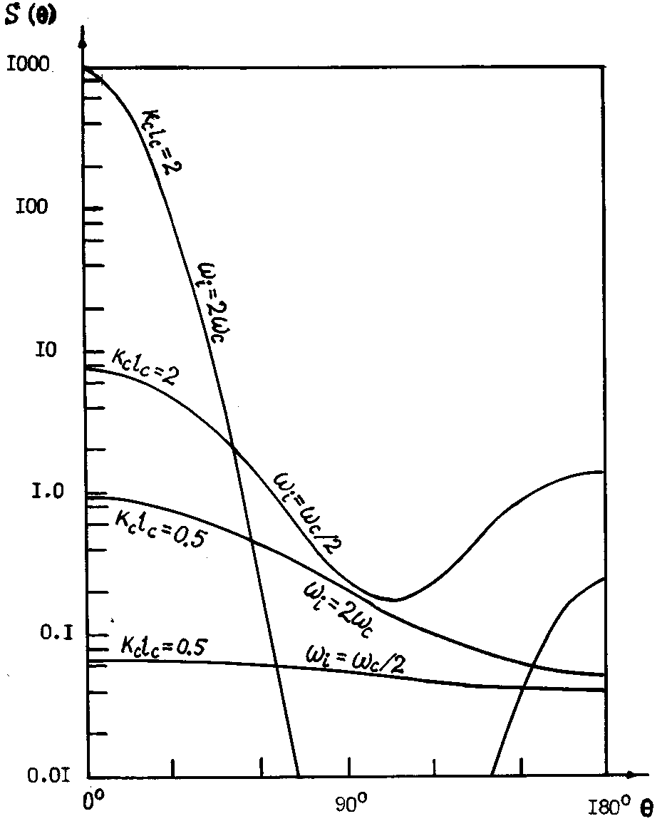Figure 2. Angular distribution of scattered sound field intensity factor [15] of full-blown turbulence region for various incident wave frequency relationships with characteristic correlation function frequency for various parameter values

Most logically current state of isotropic turbulence sound scattering theory is presented in fundamental monograph[15]. Like in[1, 4], scattering problem there is solved in Born approximation. Three types of turbulent fluctuations – compressibility, density and velocity fluctuations are considered. Though it is supposed that all fluctuation types are statistically independent, their characteristic space and time correlation radii are considered to be close. It is taken into account that for, density and compressibility flow fluctuations are of an order of in Mach number, so that their average squared values could be neglected with respect to turbulent velocity fluctuation squared value. Fig.2 shows scattered by turbulence sound field intensity angular distribution[15]. Total sound field intensity to be observed at angle, was defined by expression

,

where values of function are shown on ordinate axis of Fig.2. It is denoted - turbulent flow region volume, - observation point distance, - incident sound wave amplitude, - media density and sound velocity. Fig.2 shows data for several relationships of incident sound wave frequency with correlation spectrum characteristic frequency corresponding to correlation time, and several parameter values. Results of this study evidence that turbulence velocity fluctuation scattering maximum is always predicted in forward direction at for any parameter relationship. It is in contradiction with conclusion of[4], provided for homogeneous turbulence. Scattered field frequency dependence in high frequency limit at is the same as (1) - . And vice versa at, in low frequency limit. It rather supports Zieg experimental data than expression (10), used in for their explanation[1]. As we have already noted – the reason is in turbulence correlation function form used there. The only thing looking a little surprising is perceptible intensity predicted in backward direction – at authors of[15] opinion (c.f. Fig.2) backward intensity () is comparable to forward intensity (). As we shall see below (28), backward scattering in unbounded media for various localized flows (say, free turbulence or a set of vortices) at small M values is impossible. It is predicted in the presence of boundaries due to wave reflections only, but it is not the case studied in[15]. The problem of sound attenuation in turbulent medium was not stated in[4, 15] and evaluation of factorwas not provided.

Monograph[18] cites[4, 13], while turbulence sound scattering description is also based on two velocity fluctuations correlation function models (exponential and Gauss type). It is noted that not only inertial turbulent fluctuations interval is to be taken into account in scattering study. Importance of viscose interval described by Kolmogorov or Karman spectrum is underlined. Fig.3 shows structure of spectrum describing distribution of sound refraction index over inverse turbulent fluctuation scale. Distribution behavior in so called energetic or outer turbulent fluctuations range (general expression for it is not known) is depicted on Fig.3 by number 3. Well known dependence of in turbulent fluctuations inertial range, where - by number 2. In turbulent fluctuations viscose range where viscose losses exceed turbulent fluctuation kinetic energy dependence of is depicted by number 1[22].

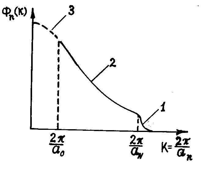Figure 3. Kolmogorov’s turbulence spectrum, describing fluctuation (vortices) intensity distribution over vortices inverse sizes space[18]

Introduction of structural empirical factors in expressions for Karman spectrum related to “weak” and “strong” turbulence respectively is of importance in[18] as well. It follows directly from turbulent fluctuation experimental data and corresponding factor values are characterized by two-order difference. In sound scattering alternative model to be proposed below this difference is derived analytically (39), (40).

Experimental study[19] in fact also cites[4], but notes undoubtedly - wind turbulence property to concentrate scattered sound presumably in forward hemisphere, not scattering practically in transverse and backward directions. In the frames of model of scattering to be developed we shall support these experimental data analytically for continuous flows (31) of non-zero vorticity.

4. Moving Media Scattering

Sound scattering crossections for various types of inhomogeneities[23-27] involved in chaotic motion were evaluated in[32] by means of averaging them with respect to sound wave incidence angle. Let us mention basic results of these works excluding corresponding solid bodies’ contributions and taking into account relationship introduced above, for several scatterer types. For instance, in[23] we have found - partial contribution of potential flow around sphere moving in ideal fluid in total scattering crossection

(11)

Similar to sense bears crossection derived in[25] for acoustically “transparent” body moving in ideal fluid, body for which density and compressibility characteristics are the same as in ambient fluid (ρ = , с = ). It is equal to

(12)

and comparable with expression (11) for partial flow scattering crossection. It is exactly the physical object taken as basic in qualitative model of moving spherical structure (fluctuation) in corpuscular model of “weak” turbulence. This element moving to the right with ambient flow lines is shown on Fig.4.

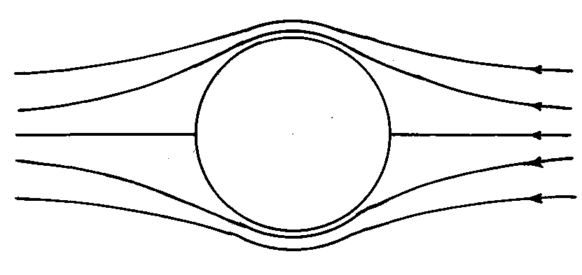Figure 4. Model of “weak” turbulence structure element - acoustically transparent moving sphere. Substance inside element has the same values of as outside. All scales of turbulence corpuscular structure chaotically moving elements from outer to inner are presented[5]

For viscose flow in the vicinity of moving inhomogeneity (particle) at, sound scattering crossection value depends on M and relationship[28-32], but for it is possible to derive. This expression is independent on moving particle contribution being the same for and in the absence of solid particles, while explicit dependence of onat in viscose media is absent. However, we are interested in microinhomogeneous media cases where viscosity influence could be safely neglected with respect to definite structure inertia. That is why expression could be used for inner minimal (Kolmogorov) turbulence scale at only[2-3, 6, 13 and 22]. With Reynolds number increase flow around spherical structures (inhomogeneities) achieve laminar wake regime[2-3, 5-6, 27 and 29-32].

In large Reynolds number range specific for turbulent media motion at two main factors are responsible for scattering – the volume of individual moving inhomogeneity (structure) itself and laminar wake behind it. It is worth to note that to eliminate divergence in wake scattering evaluation[29] we recourse to integration region restriction by physical wake length. Divergence of zero angle scattering amplitude was eliminated there by formal introduction of finite wake length L. It was shown that resulting wake scattering amplitude exceeds basic potential flow around the sphere amplitude in times[28-29]. So that at and, expression for sound scattering crossection of solid particle moving in viscose media with laminar wake generation at was

(13)

where - the value of space averaged function, while - factor depending on wave incidence angle and flow Reynolds number Re. Its explicit expression is derived in[29]. In general case however - is a factor dependent on and equals to unity in an order of magnitude. If solid particle is absent or replaced by vortex then crossection dependence is transformed to, because arbitrary flow (say, wake or vortex) scattering amplitude has the form, while in the presence of solid particle it is. Total expression for could be either the result of flow and particle contributions or - two types of flow contributions. Second case leads to expression with proportionality members only, being neglected in derivation of (13)[29], while in that case takes the form

(13a)

where - the value of angle averaged function , factor depending on wave incidence angle and flow Reynolds number Re. Factor in (13а) bears a close analogy to factor в (13). The only difference of with respect to - the latter is not restricted to unity in an order of magnitude.

At the monopole type of fluid flow outside wake is mainly responsible for sound scattering. Its contribution comprising three main components[27-30 and 32], exceeds particle and wake contributions. Corresponding angle averaged crossection expression for chaotic flow motion could be reduced to the form

(14)

Its frequency dependence is weaker than in (1), (10), and (11) and, in fact, its value is explicitly dependent on through [2]. In[29] constant value equal to unity was taken for [3], but values can decrease down to 0.2 for larger [2].

All results cited above[26, 32] are valid for structures provided by solid chaotically moving particles or derived in conditions where motion inside inhomogeneity is somehow “frozen”, for instance (10). Expression (11) - (14) comprise weak enough components related to backward scattering generated by flows around moving inhomogeneity or reflected by its surface. For “full-blown” turbulence inhomogeneity structure changes and scattering crossection expressions should be further specified.

The aim of the paper is development of alternative turbulent media sound scattering model based on spherically symmetric moving gas dynamic structure sound scattering problem solution, for instance, localized vortex problem and generalization of scattering attenuation laws on the basis mentioned.

5. Localized Flow Scattering

Let us single out stationary flow class to be used in turbulence scattering model development. Let us consider that spherical structure of radius а arbitrary related to sound wavelength is moving in the fluid. Sphere velocity V and ambient flow velocity are constant and small with respect to sound velocity с. For generality sake, let us suppose that inner sphere substance acoustic properties are possible to coincide or differ from outer flow properties. For potential flow in ideal fluid velocity distribution described in moving frame of reference outside sphere is given by[3, 5-6]

(15)

It is denoted here - unit vector, - radius vector in the frame of reference where moving sphere center is at rest. For viscose fluid moving at low Reynolds number, the flow is described by stationary Navier-Stokes linearized equation. After application of operation to both side of equation it is reduced to simple equation. Vortex flow around sphere moving with constant velocity in viscose fluid is described with aid of vector potential А. On the basis of symmetry requirements it could be evaluated through scalar function depending on scalar argument r by means of simple relationship [3, 5-6]. Using this relation together with expression for flow velocity, equation could be rewritten in the form

(16)

Various solutions of (16) for flow outside and inside sphere allow defining class of flows as a whole to which formally in particular solution (15) for is included. Using sphere center velocity finiteness, we can solve equation (16) for to have. Corresponding flow velocity distribution is[3]

(17)

Expression (17) for flow velocity is related to moving frame of reference fasten to the sphere center, while unknown factors and are to be found from boundary conditions at . Unlike solution (15) the flow defined by expression (17), is of vortex nature and its curl is nonzero. Simple enough calculations lead to the value of its vorticity being equal to. It is worth to note, that expression (17) for viscose fluid vortex flow velocity is valid for ideal fluid as well. In fact, introducing (17) in equation, being sequential to Euler equation (after application of operation), we can see that it is satisfied identically. Solutions (15) and (17) in this case are to be sewed together on the basis of tangential and normal velocity identity at to found unknown factors and В, being equal to and. For acoustical characteristics inside and outside sphere coincidence resulting flow defines Hill vortex[5]. Velocity distribution outside sphere is potential to be described by expression (15) with vorticity, while inside vortex nucleus the flow is vortex. In accordance to (17) velocity inside sphere is equal[5]

(18)

In sphere outer region () equation (16) generalized solution taking into account that for become. In laboratory frame of reference it corresponds to flow velocity at, equal to[4]

(19)

Just like the flow inside sphere, general solution for flow outside sphere (19) is vortex and its curl equals to.

It is worth to note that for and we formally obtain velocity distribution (15) with from (19). For solid sphere and velocity distribution (17), (19) is describing in fact potential flow generated by sphere moving in ideal fluid. If absolutely rigid sphere is moving in viscose fluid so that at sphere boundary velocity coincides with sphere center velocity V, Stokes flow with factors and is obtained[3]. To obtain factors in general case of moving impedance sphere it is necessary that few conditions are to be fulfilled on sphere surface. First of all velocity normal components are to be equal and equals to. In particular it leads to pair of equations and. Secondly, velocity tangential components are to be equal, leading to equation. And at last tangential stresses components are to be equal. Satisfying these conditions leads to results for and [3]

(20)

Fluid dynamical viscosity values outside and inside sphere are denoted here as and respectively. For rigid sphere, while for homogeneous media inside and outside moving structure (say, vortex) . In the last case it follows from (20) that factors are equal to.

Returning to localized flow sound scattering problem solution we note, that as in[23-32], sound propagation will be described in the frames of Lighthill equation becoming

(21)

Details of its solution are discussed in[23]. With aid of free space Green’s function solution of equation (21) takes the form of Born’s integral. Perturbation series decomposition first term neglecting wave rescattering on moving sphere surface looks like

(22)

Integration is performed here over all regions occupied by flow. Let us consider, as usual, integral behavior in long-range (wave) field region applying standard Green function transform[7]. Resulting integral is to be calculated by parts. Required scattered field is expressed through scattering amplitude - the factor in outgoing spherical sound wave in expansion of (22), in following form

(23)

Unit vector characterizes scattered wave propagation direction, while wave vector bears the sense of “impulse” delivered to fluid by wave. Its module equals to, where - scattering angle is defined by equation.

As before[23-32], integration by parts in right hand side second summand of (23), is performed over entire region occupied by flow. It means that in rigid sphere motion integration is performed over region where, while for liquid or gaseous drops or vortices it is performed not only for, but for as well. First summand integration in (23) is performed over far enough surfaces and over both sides of spherical surface at. Generally it can delimit flow regions with different velocities and. Far enough surface integral is reduced to zero. It is obvious for potential flow (15), where velocity decreases with distance as. For surface area is proportional to, integral is aimed to zero for. For flows described by general expression (19) velocity at decreases slower - as only and that is why integral may diverge. However, it is known[3, 6], that velocity distribution (19) is valid until distances of an order ~ only, where - flow Reynolds number. Analysis of more general equation

(24)

as compared to used above solution (19) of approximate equation, shows that far from the body at flow velocity decreases exponentially, proportionally to factor [3, 7]. That is why integral over far enough surfaces is reduced to zero in that case as well.

Integral over spherical surface reduces to zero in the case where flow exists on both side of it only. It is observed when velocity on the surface is continuous, i.e. . For the case of rigid body motion the flow is observed on outer side of the body surface () only, so that calculation show[23], that corresponding surface integral is non-zero. Resembling result is expected when tangential (or normal) velocity gap takes place on surface (say, due to mass exchange process). Integrals over inner and outer sides of sphere at will not coincide and result will be non-zero as well.

Now let us transform the only non-zero volume integral in the right hand side of (23) with aid of procedure used in[26]. It is based on identity known in theoretical hydrodynamics[5]

(25)

Substituting it in (23) we calculate volume integral by parts. Using Gauss theorem and low Mach number approximation where, we can rewrite expression (23) for f in the form

(26)

Integration in three first summands is performed as it was mentioned above over outer region of surface, for the case of rigid body motion only. In the cases of flow occupying entire space, integration is performed over both sides of surface. However in the absence of velocity gap corresponding integrals cancel each other. Expression (26) is simplified and reduced to the form

(27)

As we have already seen for localized flows generated by spherically symmetric structure motion, vorticity acquires simple enough angle dependence. With aid of it scattering amplitude angular structure could be calculated. Integral (27) turn out to be proportional to vector, while scattering amplitude is presented in the form

(28)

Unknown scalar function of is denoted here as. It follows from expression (28) that scattering amplitudef turns to zero in backward scattering where equality is valid and in the plane normal to wave incidence direction where or.

It is worth to note that scattering amplitudef vanishing in backward scattering is continuous flows occupying entire space sound scattering general property. It is specific for not only localized flows under analysis. Being held for the case of sound scattering in unbounded turbulent media[19, 26 and 30] it obviated validity of doubts in results of[15] mentioned above in Sec.3.

For evaluation of amplitude (28) angle dependence it is necessary to derive specific expression for with its argument depending itself on scattering angle. We are to substitute in (27) expressions for vorticity outside and inside sphere derived above

General expression for scattering amplitude for local flow (17), (19) acquires the form

(29)

- is spherical Bessel function. Few already obtained useful results follows from (29). For instance for Hill vortex where, and, scattering amplitude (29) acquires the form derived in[30] for the first time

(30)

It follows from (30) that in Hill vortex low frequency sound scattering amplitudef is equal to in an order of magnitude. Its behavior resembles scattering amplitude for potential flow near small rigid moving sphere in ideal fluid[23]. Turning to the low frequency limit in (30) we obtain Hill vortex scattering amplitude limiting value

(31)

It is worth to note that (31) exceeds many times (on an order) scattering amplitude for potential flow near small sphere[25], as well as scattering amplitude for “transparent” body. Hill vortex scattering crossection is to be calculated by standard method on the basis of (31). After simple but cumbersome calculations we receive

(32)

Averaging (32) with respect to sound wave incidence angle and taking into account notation form introduced above, we have

(33)

which exceeds substantially (on two orders) resembling expression for moving “transparent” body (12) and expression for scattering crossection of potential flow near moving rigid sphere (11). For (33) includes contribution of crossection (11) already, then we conclude that inner Hill vortex volume flow (18) yield up to 99% in its total sound scattering.

To generalize results for turbulent flows in final Kolmogorov scale motion and in the presence of touch we note that when and vorticity in outer sphere region is non-zero it follows from (29) that low frequency sound scattering amplitude turns out to be ()^-2 greater than in potential flow case. It is proportional toаМ and behaves as in the case of Stokes flow generated by sphere motion in viscose fluid[24].

If flow is restricted by particles surfaces or if flow velocity has the gap on the surface then surface integrals in general expression (26) are non-zero. As we have seen in that case scattering amplitude is non-zero even in the case of potential flow. To calculate integrals mentioned in general form let us introduce flow velocity on the surface as a sum of components normal and tangential with respect to surface to have

(34)

This presentation form allows to calculate integrals in (26) in standard manner either for flows situated in the region only or for flows occupying entire space and even for flow with velocity gap on surface. With aid of (22) we can derive those factors and in equality (34) in first case take the values and respectively. In second case velocity gap is presented in fact under integrals in three first summands of (26). For normal velocity component is to be continuous at (gap is not allowed) then. In relation to tangential velocity component gap using (17) and (19) we find. In calculations of surface integrals in (26) with aid of (34) we perform integration over outer surface side i.e. we consider that, where - space angle. Calculation of surface integrals leads to value

(35)

Volume integral in (27) is zero for flow generated by rigid sphere motion where,. It is result derived before in[23, 25]. We note that for small sphere in that case amplitude is in an order of magnitude. In the absence of velocity gap at, and surface integrals in (35) are equal to zero. Scattering amplitude is defined by volume integral (27) exclusively. It is worth to note that unbounded space vortex flow scattering amplitude angular structure defined by (28), generally in the presence of other scatterers and velocity gap surfaces could lose correctness. As it follows from (35) backward scattering could be observed while scattering amplitudef could be non-zero in the plane normal to wave incidence direction (at). Moreover contributions of flows in the vicinity of vortex or inhomogeneities in scattered fields could be expected. That is why observation of weak backward scattering contribution in turbulent media sound scattering is related mainly to rescattering, wake flows and passive touch influence. From our point weak backward scattering observation evidences multiplicity of chaotically moving scattering inhomogeneities (flows) contributing to scattering thus supporting corpuscular model of turbulent media developed here instead of formerly used model of sound scattering by large scale continuous flow.

6. Models of Scattering Media

Now we are to complete scattering medium model formulation. In the frame of model we suppose isotropic and homogeneous turbulence as a set of localized flows of various scales from outer to Kolmogorov’s. In basic flow disintegration on localized flows (vortices), say, of scale, chaotic fluctuations of not only the direction of average initial flow velocity are observed. In other words, scale motion is more isotropic than average flow. In the same way in scale formation from scale, fluctuations isotropy increases with a number of vortexes born, while basic flow influence decreases and so on. As a result after few “multiplication” stages turbulent flow becomes isotropic. In other words, in full-blown turbulence almost all vortex structure sets, except most large, are statistically homogeneous and isotropic. The larger basic flow Reynolds number value, the more fragmentation number with scales decreasing from until is observed. In inertial scale interval vortex structures are distinguished by dimensions and velocity directions only. They are universal for turbulent flows, because they have already “forgotten” basic flow structure, while viscose forces are still not important. In non-dissipative media where viscosity influences can be ignored basic these features of model are sufficient. However in realistic media scattering evaluation (in the presence of viscosity) numerical strength of most small inner “Kolmogorov” scale vortices will play substantial role. The only phenomenon side to pay attention for – is two turbulence models – “weak” and “strong”.

6.1. Weak Turbulence Model

In first model to be fair probably for flows with small enough initial vorticity, say, in wind tunnels or various small scale flow models[2, 6] – we use moving with velocity in arbitrary direction acoustically “transparent” sphere (12) of inertial range scale as basic structure (c.f. Fig.4). In turbulent flow region structures motion is completely chaotic and of zero vorticity while expression (3) for attenuation factorwith aid of (5), (6) and (12) takes the form

(36)

Ordinary attenuation frequency dependence is expected here as in[4, 15 and 17-22]. In principle, i-th type basic structure volume content factor - is different for various structures. They can be assumed the same and equal to unity for all scales in simplest case of full-blown homogeneous isotropic turbulence however. Numbers Mandunder summation sign and scale, are related to basic flow and supposed to be known.

6.2. Strong Turbulence Model

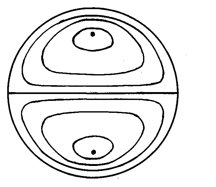Figure 5. Model of “strong” turbulence structure element - spherical Hill vortex.[5]. Substance inside element has the same values of as outside. All scalesof chaotically moving elements - from outer scale to inner scale represent turbulence corpuscular structure

In second model of “strong” turbulence to be fair probably for flows with considerable initial vorticity, say, in large scale jet flows or in reality as experimenters put it[2, 6] -– we use moving with velocity in arbitrary direction Hill vortex (33) of inertial range scale as basic structure. Its inner flow is shown qualitatively on Fig.5. As before for “weak” turbulence model – all scales of such elements from outer to inner (Kolmogorov’s) are present in model.

Moving to the right “strong” turbulence model basic element (spherical Hill vortex) meridian plane hydrodynamic velocity field lines are shown on Fig.5. Characteristic parameters of substance inside vortex coincide with outside parameters. It ensures basic structure acoustic “transparency” and thus scattering is provided by fluid flow inside and outside structure only. Vortex lines are situated in the planes normal to structure symmetry axis. Flow velocity field lines are tightened around thick points on Fig.5[5]. In that case fluid flow in turbulent volume is partly vortex (inside vortexes) completely chaotically and expression (3) for attenuation factor with aid of (5), (6) and (33) takes the form

(37)

Expressions (36) and (37) resemble in structure and frequency dependence, but their magnitudes differ in two orders due to inner vortexes part contributions specific for “strong” turbulence model. Difference in turbulent fluctuations intensity between laboratory wind tunnel model and realistic flows in an order or more is observed in experiments[2, 6, 12 and 18]. Probably, such relationship could be expected for corresponding sound scattering results as well. However experiments on their comparison are not known to author.

It is known, that even in inertial scale ranges of basic structures motion in dissipative medium (in the presence of viscosity) fluctuation characteristics differs substantially from observed in ideal fluid. First of all they are characterized by wakes with contributions (13) and (13a) and by generation of additional flows outside wakes with contribution (14) to total sound scattering. Furthermore in dissipative media scattering evaluation numerical strength of most small inner “Kolmogorov” scale vortices will play substantial role. They scatter sound in accordance to structure motion in viscose media with scattering crossection [24] in conditions where structure inertia is to be neglected. Kolmogorov’s vortexes volume fraction can be taken equal to unity for preliminary evaluation. Large Reynolds number flows sound scattering was studied in[27-30 and 32] and it was shown that scattered sound structure and spectrum are dependent on relationship of structure Mach number and wave dimension in inertial scale range. At least three cases are available.

In first case at and, low frequency sound wave is scattered in inertia structures scale range. Vortex flow outside wake is responsible mainly for sound scattering defined by first monopole summand of (19). Hill vortex (33) is used here as a basic structure with dimension belonging to inertial scales interval and moving with velocity in arbitrary direction. Resulting flow is vortex (inside vortex volumes and partly outside wake) and completely chaotic. Expression (3) for attenuation factor allowing for sound scattering by Kolmogorov’s scale turbulence with aid of (5), (6), (33) and (14) takes the form

(38)

Notation «» in (38) indicates influence of monopole type flow outside wake.

In second case atslightly higher frequency sound wave is scattered in inertial turbulence scale where inner structure volume and laminar wake beside it are responsible for scattering. Hill vortex (33) is used here as a basic structure with dimension belonging to inertial scales interval and moving with velocity in arbitrary direction. Resulting flow is vortex (inside vortex volumes and partly inside wake) and completely chaotic. Expression (3) for attenuation factor allowing for sound scattering by Kolmogorov’s scale turbulence with aid of (6), (8), (33) and (13a) takes the form

(39)

Notation «» in (39) indicates influence of moving vortex wake.

In third case, for given sound frequency in turbulence inertial scale range first case of scattering is observed in definite range part, while second case of scattering is observed in reminder part. Hill vortex (33) is used here as a basic structure with dimension belonging to inertial scales interval and moving with velocity in arbitrary direction. Resulting flow is vortex (inside vortex volumes, inside wake and partly outside wake) and completely chaotic. Expression (3) for attenuation factor allowing for sound scattering by Kolmogorov’s scale turbulence with aid of (5), (6), (33), (13a) and (14) takes the form

(40)

Natural number corresponds to sum term number for which at definite relationship is attained. In other words, related to turbulence scale. It is worth to note passive touch (say, dust) role in sound scattering – it is more noticeable in particles scale range. Finer scale touch particles have negligible influence on total scattering. Quite the contrary, when condition is valid total sound attenuation factor can change from the form (16а) - , at least partly to the form (13) - , providing more intensive sound wave scattering.

7. Discussion

Thus, in general, for touchless turbulence, attenuation factor spectrum in realistic viscose turbulent medium depends on frequency in the following manner. At lowest frequencies as well as for small M, key contribution to total attenuation provides scattering of sound by Kolmogorov’s turbulence scale. It is independent of frequency and provides definite attenuation spectrum pedestal. Further on with frequency increase at attenuation component related to scattering on flow vorticity outside moving structure and structure wake come into force. This spectrum component increases with frequency squired until scales where. And, at last, at attenuation component related to scattering inside moving structure wake and volume come into force. This spectrum component increases with frequency fourth grade until for scales up to , if for sure. These laws are partly different from well-known propositions of wave turbulence scattering theory[1, 4, 15 and 17-19]. Moreover, mentioned component relationship (40) depends additionally on a set of internal problem factors, say, Mach number, Reynolds number and several numerical factors. It could be changed in changing conditions. That is why mentioned above Sieg experiment results[1, 33] for small M look understandable. They rather allow discussing turbulent flow structure in experiments. Preliminary quantitate estimates are performed on the basis of spectrum pedestal mentioned above . In fact, in Sieg experiment frequency range 250 – 4000 Hz[1, 33-34], condition is to be met even for outer turbulence scale. So that should be of an order of 10^-2 m. At contributions of second () and third () summands of (40) are to be neglected with respect to contribution of (). To evaluate boundary frequency value it is of use to note, that expression for is derived with aid of (21), in condition where flow is described by equation (16). That is when it is possible to neglect partial time derivative in (16) in expression for total derivative[28, 32]. In other words when flow vorticity exceed characteristic incident sound frequency. Estimates on the basis of vorticity expression for outer atmosphere turbulence scale and wind velocities in Sieg experiments lead to frequency boundary value of an order 150 – 250 Hz[33].

For wind velocity in interval 1 - 2 m/s, Reynolds number, Mach number squared, give for m^-1. Resulting attenuation is close to value 1 – 1.5 dB at 100 m, as in Sieg data[1, 33-34], without frequency dependence of. For wind velocity increase up to 10 m/s at frequency 250 Hz taking into account outer scale increase we obtain m^-1, attenuation close to 7 dB at 100 meters. Further increase of with frequency and wind velocity observed in experiment coincides with law (40) accounting for spectra and . It evidences qualitative coincidence of proposed model predictions with experiment.

Typical attenuation factor frequency (wave parameter) dependence derived in the frames of corpuscular turbulence scattering models for “weak” (curves 1, 3) and “strong” (curves 2, 3, 4, 5) turbulent media are shown on Fig.6. Dependence related to well-known turbulence wave model[4, 18] – curve 6 while crosses[1, 33] show Sieg experiment results.

It is seen that available experimental data on sound attenuation in atmosphere are explained by proposed “strong” turbulence scattering corpuscular model (zero frequency power dependence, ), while known wave models in low frequency range (fourth frequency power dependence, ) are at noticeable variance with experimental data.

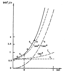Figure 6. Typical sound attenuation index (multiplied by 103) frequency (wave number parameter) dependencies developed in the frames of atmospheric turbulence scattering corpuscular models for strong (curves 2, 4, 5) and weak (curve 1) turbulent wind flow regimes[30]

8. Conclusions

As a general paper result we can conclude:

It is recommended to use in turbulent media low frequency sound scattering and attenuation modeling “corpuscular” model of scattering developed in the paper. The model comprises media as a set of chaotically situated and moving localized flows of various scales. Both inner and outer flow parts are responsible for scattering.

In the absence of boundaries scattering amplitude of arbitrary continuous flow (say, turbulent flow) for arbitrary relationship of characteristic scale to sound wavelength is defined by flow vorticity and turns to zero for backward scattering and for scattering in the plane normal to wave incidence direction.

For further sound scattering and attenuation modeling applications we can recommend to take into account specific features of model:

Turbulence non-dissipative attenuation factor frequency spectrum acquires ordinary Rayleigh law form- the same form as in known turbulence sound scattering models. Spectrum increases with fourth frequency degree until up to scale, if.

Normalized factors for corpuscular models of “strong” and “weak” turbulent media differs in two orders due to contribution of inner flow in “strong” turbulence scattering model, but for low frequency sound scattering at low Mach number both models are to be provided with contribution of viscose flow corrections scattering.

Corrections to attenuation factor spectrum related to viscosity influence depend on frequency in the following way. In low Mach number low sound frequency case defining contribution is provided by sound scattering on Kolmogorov’s scale turbulent fluctuations. It is perceptible in any frequency range providing a kind of pedestal for attenuation spectrum. Then with frequency increase at, spectrum component related to vorticity outside model structures and their wakes come into force. This spectrum component increases with frequency squared in scale range until scales. And, at last, at spectrum component related to vorticity inside model structures and inside their wakes come into force. This spectrum component increases with frequency fourth degree in scale range until up to scale, if.

Passive touch (say, dust) contribution to turbulence sound scattering – is most perceptible for particles scales in the range. Finer scale touch particles have negligible influence on total scattering. Quite the contrary, when condition is valid total sound attenuation factor can change from the form, at least partly to the form, providing more intensive sound wave scattering.