-
Paper Information
- Next Paper
- Previous Paper
- Paper Submission
-
Journal Information
- About This Journal
- Editorial Board
- Current Issue
- Archive
- Author Guidelines
- Contact Us
American Journal of Fluid Dynamics
p-ISSN: 2168-4707 e-ISSN: 2168-4715
2012; 2(6): 101-116
doi: 10.5923/j.ajfd.20120206.03
Stochastic Large Eddy Simulation of an Axisymmetrical Confined-Bluff-Body Particle-Laden Turbulent Flow
 Abstract
 Reference
 Full-Text PDF
 Full-Text HTML
Abdallah Sofiane Berrouk
Department of Chemical Engineering, The Petroleum Institute, Abu Dhabi, P.O. Box 2533, United Arab Emirates
Correspondence to: Abdallah Sofiane Berrouk, Department of Chemical Engineering, The Petroleum Institute, Abu Dhabi, P.O. Box 2533, United Arab Emirates.
| Email: |  |
Copyright © 2012 Scientific & Academic Publishing. All Rights Reserved.
Flow turbulence modulation by dispersed solid particles in a bluff body was studied using two-way-coupled stochastic large eddy simulation. Point-force scheme was used to model the inertial particle back effects on the fluid motion. The fluid velocity field seen by inertial particles was stochastically constructed based on the filtered flow field obtained from well resolved large eddy simulations. For that purpose a Langevin-type diffusion process was used with the necessary modifications to account for particle inertia, cross-trajectory effects and the two-way coupling. The numerical results regarding mean and turbulence statistics for both phases show a very good agreement with the experimental findings for both light and heavy mass loadings (22% and 110% respectively). This numerical investigation demonstrates also the ability of the stochastic-LES-particle approach to predict turbulence modification by inertial particles.
Keywords: Gas-Particle Flows, Large Eddy Simulation, Eulerian-Lagrangian, Turbulence Modulation, Point-Force Coupling, Stochastic Modeling
Cite this paper: Abdallah Sofiane Berrouk, "Stochastic Large Eddy Simulation of an Axisymmetrical Confined-Bluff-Body Particle-Laden Turbulent Flow", American Journal of Fluid Dynamics, Vol. 2 No. 6, 2012, pp. 101-116. doi: 10.5923/j.ajfd.20120206.03.
Article Outline
1. Introduction
- In turbulent dispersed flows, particles are driven by the carrier phase and as a consequence this phase experiences reaction forces from these particles. The contaminating character of particles locally modifies the turbulence, since inside the particle there is no flow field and no eddies. This kind of local modification is expected to be negligible if the particle diameter is much smaller than the Kolmogorov scale[1]. However, when higher particle loadings are considered (volume fraction
 > 10-6), particles significantly affect the turbulent flow field and the two-way coupling between the phases has to be taken into account.The presence of particles in a turbulent flow can modulate the turbulence in several ways. Particles can distort streamlines or modify velocity gradients leading to a change in turbulence generation.Large particles can generate wakes yielding a turbulence enhancement while small particles cause turbulence damping by the drag forces on them since kinetic energy is converted into heat. This has been the general trend shown by the experimental data[2-5] based on which many demarcation criteria for attenuation or enhancement of gas turbulence in the presence of particles were proposed[6-9]. With the steady increase in computing power, there have been numerous efforts to numerically quantify turbulence modulation by inertial particles. However, highly resolving the flow around thousands to millions of particles to get an accurate particle/turbulence interaction has been prohibited by the number of grid points required. Eaton and Segura[10] showed that one million grid points is needed to mesh a local spherical grid of diameter equal to 25dp to keep errors, in comparison with high-resolution experiments, under 1%. Thus, physical models have been developed and “plugged” to well-resolved numerical simulations to render prediction of turbulence modulation tractable. A commonly applied model is the point-force model that was first used by Squires and Eaton[11] and subsequently improved bySundaram and Collins[12] and Lomholtet al.[13]. The point-force scheme was originally an adaptation of the Particle-source-in-cell (PSIC)[14]. As stated by Eaton and Segura[10] , the point-force model, when added into a Direct Numerical Simulation (DNS), is believed to capture the effects of particles on the energy-containing eddies while being incapable of capturing the extra viscous dissipation associated with the small-scale-turbulence/particle interaction. It is then expected that this fact will be exacerbated when the point-force model is used in the context of Large Eddy Simulation (LES) where the small-scale or the sub-grid-scale motion is discarded by the spatial filtering operation inherent in LES calculations. Segura et al.[15] performed a well-resolved LES of a channel flow using the point-force coupling model. The single-phase flow and particle motions for light loading cases (mass loading ≈ 20%) were accurately predicted compared to the experimental results of Paris and Eaton[16] where as the turbulence attenuation was grosslyunder-predicted. There are some reasons behind the failure of the point force scheme to capture the high levels of local dissipation around the particles. One reason is that most of the Lagrangian models relate the particle drag to the undisturbed fluid velocity which is not available in a two-way coupled LES. The undisturbed fluid velocity field is defined as the velocity field that would exist if the particle was not present. Another reason is the under-prediction of particle drag by Lagrangian tracking models because the models do not account for the effects of subgrid scale turbulence that is missing in the LES field. Thus, the representation of the extra dissipation that occurs at the sub-grid scales may yield amelioration of the point-force LES predictions for Lagrangian two-phase flows.In recent reviews on two-way coupled turbulencesimulations of gas-particle flows, Eaton[17] and Balachandar and Eaton[18] acknowledged the shortcomings of the point-force model in accurately capturing particle-turbulence interaction. They suggested the development of LES with a sub-grid scale model that is locally modified by particles since high-resolution numerical simulations of particle-laden flows are still beyond hope. This suggestion is in line with the outcomes of Elghobashi[19] work who pointed out that in case of a significant two-way coupling, the sub-grid scale turbulence model might need modification specifically if the particulate phase couples strongly with the small scales turbulence (matching between the particle and the sub-grid scale turbulence time scales). Thus, the two-way turbulence modeling should be carried in a rigorous way that account for the particle presence. However, it is well known that there is no precise ‘geometrical’ knowledge on the structure of turbulence in the presence of a suspension of discrete particles and this makes it extremely difficult to modify the one-way turbulence modeling as well as the theory of Kolmogorov on which many turbulence closures for two-phase turbulent flows are based. In the case of two-way coupling, it is assumed that the presence of solid particles changes the transfer rates of energy and energy dissipation while the nature and structure of turbulence remain the same[20]. This implies that one-way turbulence models can be used for two-phase turbulent flows after taking into account the fluid-particle coupling through the void fraction. However, Boivin et al.[21] indicated that the presence of particles in isotropic turbulence yield a non-uniform distortion of the energy spectrum. Squires and Eaton[11] demonstrated that the non-uniform distortion is dependent upon the particle relaxation time. In a different work by Squires and Eaton[22], the non-uniform distortion of the turbulence energy spectrum by particles was attributed to preferential concentration. Also, Elghobashi and Truesdell [23] found that the coupling between particles and fluid yielded an increase in small-scale energy. The relative increase in the energy of the high-wave-number components of the velocity field resulted in a larger turbulence dissipation rate. They also stated that the effect of gravity caused an anisotropic modulation of the turbulence and an enhancement of turbulence energy levels in the direction aligned with gravity. All these findings point towards the fact that the nature and the structure of the energy transfer mechanisms of turbulence are modified by the presence of particles. In this case, modeling of the energy dissipation has to be altered in a manner that takes into account such a modification in turbulence structure. However, the empirical input required for both Reynolds-averaged and LES approaches at the present time makes it difficult to obtain a rigorous two-phase turbulence modeling as suggested by Eaton[17]. Due to this severe limitation, LES modeling of two-waycoupled particle-laden turbulent flow using the point-force scheme should ideally include the sub-grid turbulence motion as seen by the inertial particles. The stochastic approach based on Langevin equation emerges as a promising candidate in this regard. Previous numerical investigations by Berrouk et al.[24, 25] and Berrouk and Laurence[26] in the context of one-way coupled gas-particle turbulent flows showed its promising potential in accounting for the effects of sub-grid turbulence motion on inertial particle dispersion and deposition. In the present work, a Langevin-type diffusion process is used in conjunction with Lagrange LES as a tentative model to compute mean, turbulence statistics and turbulence modulation as predicted by the experimental work of Borée et al.[27] on gas-particle turbulent flow in a confined bluff body. The experiment of Borée et al.[27] presents a challenging validation case for the stochastic Lagrangian particle-LES model since it contains multiple complex flow features such as strong recirculating zones created by dump geometry and multiple stagnation points beside the high Reynolds number. This configuration is typical of an industrial application where the objective is to control the mixing of a fuel (pulverized coal) with the air. Minier et al.[41] showed the potential of RANS/PDF approach through the simulation of the experiment of Borée et al.[27]. Riber et al.[28] simulated the experiment of Borée et al.[27] for the light mass loading case (M=22%) using both hybrid and Lagrange LES. They investigated the effects of the numerical schemes, gas and particle boundary conditions, the grid refinement and the sub-grid scale models on the particle-LES accuracy and they confirmed the potential of LES approaches for two-phase turbulent flows and their relative insensitivity to the details of the numerical solver. Moreover, they recommended accounting for the effects of subgrid fluid turbulence on the particle dynamics which is particularly crucial for the heavy mass loading case.
2. Problem Formulation
2.1. Governing Equations for Fluid Flow
- The equations for the carrier fluid flow are solved using the LES methodology. The LES model is based on spatial filtering of the velocity field:
 | (1) |
 plays the role of a low-pass filter that eliminates scales smaller than the filter width
 . This results in smoothing the signal u which is usually random and unpredictable. The velocity can be decomposed into resolved and sub-grid scale components:
 | (2) |
 | (3) |
 | (4) |
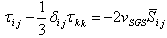 | (5) |
 is the subgrid-scale viscosity:
  | (6) |
 , where
  is the resolved rate-of-strain tensor. The value of the constant
  is evaluated based on the dynamic procedure[30, 31]. The filter width,
  is taken equal to
  with
with  is the cell volume.The two-way coupling effects are incorporated in the form of a reaction force exerted by the particles on the fluid. This reaction force is equal and opposite to the sum of fluid forces, only drag force in the present simulation, acting on the particles. Therefore the source term
 in the momentum equation is given by:
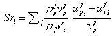 | (7) |
 and
and are the volumes of the cell and solid particles, respectively.
  is the velocity of a given particle p and
  is the fluid velocity seen by the particle p along its trajectory. It is computed based on the resolved velocity using a stochastic diffusion process as we shall detail in the next section.
 2.2. Governing Equation for Particle Motion
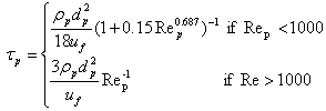
- The particle motion is calculated in the Lagrangian frame of reference. This approach requires interpolation of the surrounding carrier fluid velocity ūi onto the particle position. This was done using a tri-linear interpolation scheme. The particle motion in the Lagrangian frame of reference is described by the following set of equations[32]:

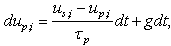
 | (8) |
 is the particle position, g is the gravity force per unit of mass,
  and
and  are the diameter and the mass density of inertial particles,
  is the particle response time
  is the particle Reynolds number:
 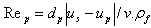 and ν are respectively the density and the kinematic viscosity of the fluid. The effect of particle-particle collision is neglected for these simulations because it is deemed that the momentum exchange due to p-p collisions is much smaller than the momentum exchange due to the forces exerted by the gas since the volume loading ration is still below values usually characterizing contact-dominated flows. We shall discuss this point later in more details.The unknown in the system of Eqs. (8) is the fluid velocity
  seen by inertial particles along their trajectories as they move through the turbulent field. The Eulerian velocity field computed using Equations of section 2.1 and interpolated to the particle positions, contains only part of the information of the velocity field that inertial particle should see. This information is linked to the filtered velocity of the large scales. Any information about the sub-grid scale motion is lost because of the filtering operation. This information on the turbulence at the subgrid scale level is crucial for the transport of inertial particles with response times smaller than the smallest LES-resolved time scales. The Langevin model can be used to reconstruct the Lagrangian instantaneous fluid velocity increment as seen by inertial particles based on the LES filtered velocity. The model should account for the inertial character of the particles and the presence of a body force. The general form of the Langevin model chosen for the velocity of the fluid seen by particles is:
  | (9) |
 and the diffusion matrix
  have to be modeled. Each component of the vector dW is a Wiener process (white noise); it is a stochastic process of zero mean,
  a variance equal to the time interval,
  and delta-correlated in the time domain[33].The theoretical and numerical formulations of the Langevin model have been extensively discussed in the framework of particle-laden RANS[34, 35]. The use of the Langevin model was extended by Berrouk et al.[24] for the modeling of time increment of the fluid velocity seen by inertial particles in LES framework. A detailed derivation of the different terms of the Lagrangian model is provided by Berrouk et al.[24, 26] for the case of one-way coupled LES. Hereafter, we shall discuss only the evaluation of Langevin equation’s terms in the case of inhomogeneous and anisotropic turbulence and how to account for particle inertia, cross-trajectory effects (CT), and the two-way coupling. For two-way coupled situations, the Langevin equation reads:
 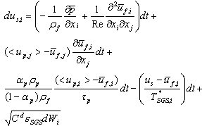 | (10) |
 is the fluid velocity seen by particles along their trajectories,
  is the fluid SGS time scale seen by particles,
  is the diffusion constant and
  is the dissipation rate of the SGS kinetic energy
 . The fluid SGS time scale seen by inertial particles
  is
is  (the Eulerian SGS time scale) in the limit of large Stokes number. if
 reduces to
  (the Lagrangian SGS timescale) since in this case the inertial particles reduce to fluid elements. Thus,
  is in general a function of
  and varies between
  and
and  as it is portrayed in the following equation[36]:
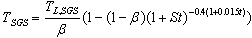 | (11) |
 is Stokes number based on the Eulerian SGS time scale and
  is the ratio between the Lagrangian and the Eulerian time scales. It is assumed that
  keeps the same value across the different scales of turbulence:
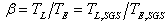 | (12) |
 is chosen to be 0.356[36]). Eq. (11) was developed for particles interacting with homogeneous and isotropic turbulence. Its use in the present context to account for inertia effect on Lagrangian subgrid time scale is more appropriate compared to its use to include inertia effect on Lagrangian time scale in the framework of RANS/SM where the construction of a wide spectrum of anisotropic turbulence fluctuations is sought through the stochastic modeling. For LES, the Lagrangian time scale for the sub-grid fluctuations
  is computed using the sub-grid kinetic energy
  and its dissipation rate
  . The last two quantities are evaluated according to the SGS model used to take into account sub-grid effects on the large scales. It reads following Heinz[38]:
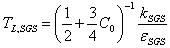 | (13) |
 | (14) |
 and the Kolmogorov constant is taken equal to 2.1[39].The directional dependence of the fluid Lagrangian SGS time scales
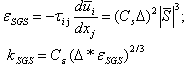
  is neglected since sub-grid scales are assumed to be homogeneous and isotropic. To account for the cross trajectory effect due to the presence of a body force, the Lagrangian time scale is expressed in the case of inertial particle as function of the instantaneous relative velocity between the fluid and the inertial particles[20]. If we assume direction (1) is the one aligned with the direction of the mean relative velocity and (2) and (3) are the transversal ones, we can use Csanady formulas[40] to compute the different anisotropic time scales:
 | (15) |
 is the mean slip velocity between fluid and inertial particles. k is the resolved turbulent kinetic energy. In fact, Csanady formulas[40] also take into account the continuity effect. The continuity effect postulates that the inertial particle dispersion in a direction perpendicular to the mean drift is twice as faster as inertial particle dispersion in a direction parallel to the mean drift. The diffusion coefficient
  is evaluated according to the following formulation[20]:
 | (16) |
 is the modified SGS kinetic energy:
 | (17) |
 is the fluid fluctuating velocity and
  , (i=║or ┴) The mean statistical behavior of the cloud of particles that is present in one cell at time t should be taken into account. This results in an additional term in the equation of the drift[20]. In the fluid case, the drift term entering the stochastic differential equation is chosen to be a sum of a filtered term and a subgrid fluctuation term that is characterized by a time scale
 . This form is retained for thetwo-phase flow case with a modification of both altered and fluctuating terms to account for the inertia and cross trajectory effects. In case of two-way coupling, it is assumed that solid particles impact the turbulent kinetic energy transfer rate and dissipation with a little effect on the nature and structure of turbulence. Based on that assumption, Minier et al.[20, 41] proposed a model for the seen fluid velocity in case of two-way coupling in RANS framework. They added a source term to the mean part of the drift term to account for the two-way coupling situations. This idea is retained for the LES calculations and depicted by adding the extra acceleration term in Eq. (10).
3. Numerical Simulation Overview
- A flow solver from the R&D section of Electricite de France named Code_Saturne (www.code-saturne.org) was used to simulate Borée et al.[27] work. The discretization in Code_Saturne is based on the collocated finite-volume approach. It allows solving Navier-Stokes and scalar equations on hybrid and non-conform unstructured grids. Velocity and pressure coupling is ensured by a prediction/correction method with a SIMPLEC algorithm. The collocated discretization requires a Rhie and Chow interpolation in the correction step to avoid oscillatory solutions. A second order centered scheme (in space and time) is used. The flow solver has been extensively tested for LES of single-phase flows[42, 43]. The stochastic differential equations (SDE) system that comprises Eqs. (8) and (10) is integrated using an appropriate weak second-order integration scheme[35] that accounts for the nature of the problem characterized by the presence of different time scales. This can lead to stiff equations when the smallest time-scale is significantly less than the time-step of the simulation. This point is crucial for physical and engineering applications, where various limiting cases can be present at the same time in different parts of the domain or at different times. Because turbulence problem has a multi-scale character, three time scales are considered: The observation time scale,
 , and two physical time scales, the particle relaxation time,
  , and the time scale of the fluid velocityseen,
  . When these scales go to zero, a hierarchy of stochastic differential systems is obtained. The Langevin-type model used in this study degenerates to a stochastic model for turbulent diffusion when
  approaches 0, that is, the inertial particles behave like fluid particles. The weak second-order integration scheme consists of a prediction step and a correction step. The prediction step is a weak first-order integration scheme (Euler scheme). By freezing the coefficients on the integration intervals and by resorting to Ito’s calculus, it can be shown that the SDE system (Eqs. 8 and 10) has an analytical solution[26, 35].As test case for the developed model, an axisymmetrical confined-bluff-body particle-laden turbulent flow is simulated. It consists of the experimental work of Borée et al.[27] performed using the flow loop Hercule at EDF R&D. In this experimental work, a low Reynolds number inner jet (Re ≈ 4500) laden with polydispersed glass particles interact with an outer jet characterized by a higher Reynolds number (Re ≈ 40000) creating therefore a zone of strong recirculation (Fig. (1)).
 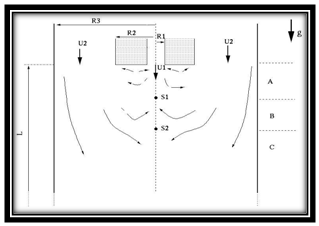 | Figure 1. Sketch of the confined bluff body flow |
 and
and  ) are kept under 5 to avoid oscillations in the gradient computations. The velocity profile at the inlet (z=-0.1 m) is prescribed by imposing the experimental mean and turbulence fluctuations measured at z=0 m. Non-slip conditions are imposed at the walls while the outlet is purely convective. A polydispersed glass particles are considered inBorée work[27] with material density (
 = 2470 kg/m3) and diameter that covers a wide range of size classes from
  to
to . Figure (4) shows the particle distribution in mass and in number. Two mass loadings are considered in this experiment and they are both high enough to give rise to a two-way coupling between the carrier and the dispersed phases. The experimental findings show that for the highest mass loading (M=110%), the turbulence is modulated by the particles to an extent that it suppressed the two stagnation points that were observed for the smaller mass loading case (M=22%) and particle-free case. The particle mean and fluctuation profiles are imposed at the inner pipe inlet (z=-0.1 m, R= 0 m) and correspond to the ones measured experimentally at z=0 m. The time step used to solve the continuous phase is ∆tf = 10-4 while the one used for the particulate phase is one order of magnitude smaller: ∆tp = 10-5.
 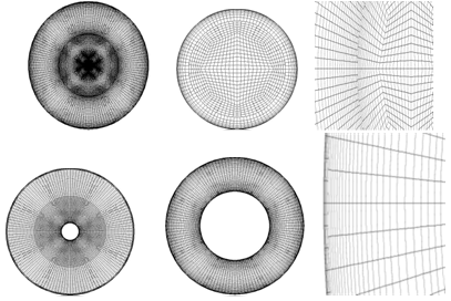 | Figure 2. Cross section unstructured mesh of the bluff body |
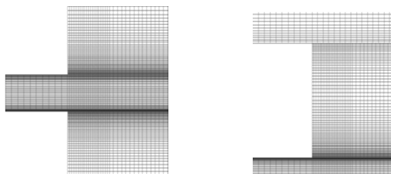 | Figure 3. Longitudinal unstructured mesh |
4. Results and Discussion
- In this section, the numerical results of the stochastic LES are compared to the experimental results of Borée et al.[27]. Experimental measurements are obtained with a Phase Doppler Anemometer and experimental data for the continuous phase of the particle-free case (M=0%), continuous and dispersed phases for the particle-laden cases (M=22% and M=110%) are available for radial profiles of different statistical quantities at different axial distances downstreamof the injection. These quantities include the mean axial and radial velocities for both fluid and particle phases. Axial profiles along the axis of symmetry for these quantities are also provided. Before detailing these results, the well-resolvedness of the present LES, justification of the use of the stochastic model,and neglect of the particle collisions are discussed. To ensure the large eddy simulation well-resolvedness, the averaged amount of the turbulent kinetic energy kSGS discarded by the grid resolution and the LES modeling shouldnot exceed 20% of the total turbulent kinetic energy according to Celik et al.[44] and Pope[45].A-posteriori estimation of the filtered out kinetic energy based on Eqs. (14) demonstrates that the present LES is adequate according to the LES index of quality[44, 45]. Indeed, the ratio of the SGS kinetic energy to the total kinetic energy (KER) is globally well under 20% almost everywhere in the domain and consequently the present LES is adequate. This fact is depicted by Figs. (5a) and (6) for the streamwise and radial directions respectively.
 | Figure 4. Initial distribution of the particle size |
 . It is defined as the ratio of the particle response time to the SGS turbulence time scale
  .
.  | Figure 5. Streamwise profiles of ratio of fluid subgrid turbulent kinetic energy to fluid total turbulent kinetic energy (KER) and subgrid time scale (TSGS) |
 | Figure 6. Radial profiles of ratio of fluid subgrid turbulent kinetic energy to fluid total turbulent kinetic energy. (a) z=0.003m; (b) z=0.08m; (c) z=0.16m; (d) z=0.20m; (e) z=0.24m; (f) z=0.32m ; (g) z=0.40m |
|
 , is estimated using Eqs. (11-13) and depicted by Figs.(5b) and (7) for the streamwise and radial directions respectively.
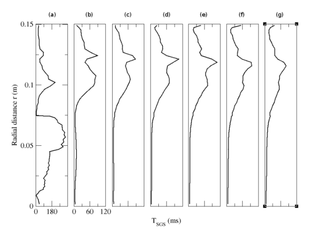 | Figure 7. Radial profiles of subgrid time scale TSGS. (a) z=0.003m; (b) z=0.08m; (c) z=0.16m; (d) z=0.20m; (e) z=0.24m; (f) z=0.32m ; (g) z=0.40m |
 .Results indicate that particles with a diameter up to
  do sense the discarded SGS turbulence irrespective of their positions in the chamber since their Stokes numbers based on the SGS time scales are smaller than one. These classes of particles represent around 35% of the number of particles injected as it is shown in Fig. (4). The transport of these classes of particles should be affected by the discarded subgrid scale SGS turbulence. Hence the effect of latter should be modelled which justifies the use of the stochastic model described above. Particle-particle collision is usually taken into account for cases where the particle volume fraction
  exceeds 10-3[18]. Present numerical results on the maximum particle volume fraction (Fig. (10a)) show that the latter has a time-averaged value of around
  for M=22% mass loading and
  for the M=110% mass loading. Figure (10b) shows that these maximum particle volume fractions
  are found for a limited number of cells equalling 0.05% of the total cell number for M=22% mass loading and 0.5% for the M=110% mass loading. Thus, an algorithm handling particle collisions was deemed not necessary. The decision of not including a time-expensive p-p collision algorithm in the present simulation is also justified by the fact that the time between successive inter-particle collisions,
  , is larger than the largest response time of all particle classes present in the chamber (see Tab. (2)), whereby the fluid dynamic transport of the particles is the dominant effect.
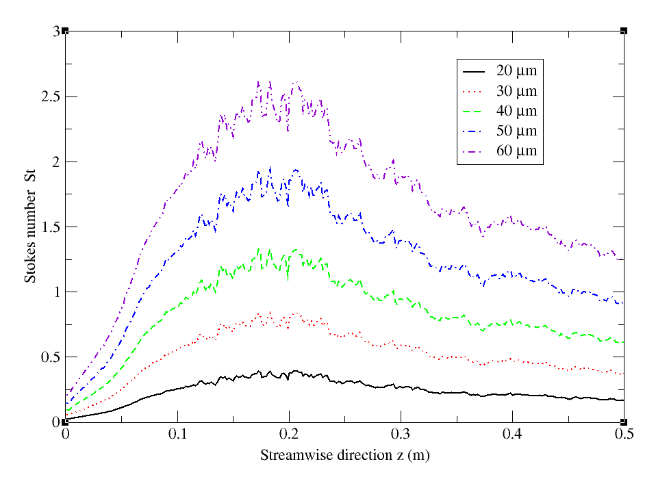 | Figure 8. Streamwise profiles of Stokes number (St) |
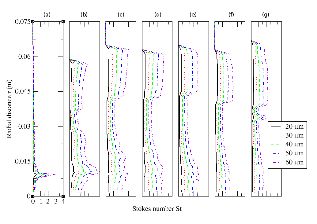 | Figure 9. Radial profiles of Stokes number (St). (a) z=0.003m; (b) z=0.08m; (c) z=0.16m; (d) z=0.20m; (e) z=0.24m; (f) z=0.32m ; (g) z=0.40m |
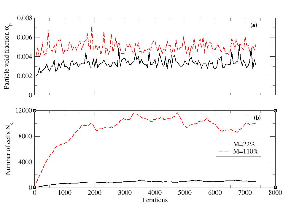 | Figure 10. Time variation of: (a) maximum particle void particle αpand (b) number of cells Nc with αp > 10-3 |
 , is computed following Lain an Garcia[46]:
 Where
Where  is the minimum (lower) particle diameter
 ,
, is the maximum (upper) particle diameter
 ,
,  is the maximum relative velocity between particles
 , and
, and  is the particle number concentration defined as particle/m3
  227 million particles/m3. The overall results regarding both carrier and particle phases obtained using the stochastic LES model and the point-force scheme to account for the two-way coupling are in good agreement with the measurements of Borée et al.[27]. In the next sections, numerical results for continuous and dispersed phases are compared to experimental findings and the effects of the mass loading on both mean and turbulence statistics of the continuous phase are discussed.
 4.1. Carrier Phase
4.1.1. Particle-Free Case: M=0%
- In the single-phase configuration, the experimental observations of Borée at al.[27] allow to schematically decompose the flow into three longitudinal regions as depicted by Fig. (1). Region A ranges from the jet nozzle to the first stagnation point S1. In this region, the jet is rapidly stopped by the recirculating flow. The central jet is surrounded by a recirculation upward flow which feeds both the initial entrainment in the jet and the annular shear layer developing at the edge of the bluff body. The positive pressure gradient due to the section increase should play an important role in the particle dispersion. Region B ranges from S1 to S2 and represents the recirculation region. An intense upward flow on the axis is detected. Profiles measured further downstream of the second stagnation point S2 show that region C downstream S2 corresponds to the development of a wake flow. In two-phase configuration, this description remains valid for low mass-loading only. It was shown that no mean stagnation points on the flow axis is detected for the M=110% case as a result of a strong two-way coupling in the dense central jet.
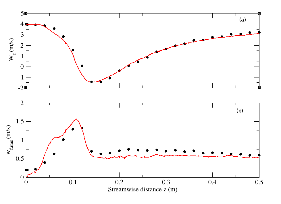 | Figure 11. Streamwise profiles of (a) fluid mean streamwise velocity and (b) fluid RMS streamwise velocity for the particle-free configuration (M=0%). Circle: Experiment; solid line: Numerical simulation |
 | Figure 12. Radial profiles of fluid mean streamwise velocity for particle-free configuration (M=0%). Circle: Experiment; solid line: Numerical simulation.(a) z=0.08m; (b) z=0.16m; (c) z=0.20m; (d) z=0.24m; (e) z=0.32m ; (f) z=0.40m |
 | Figure 13. Radial profiles of fluid mean radial velocity for particle-free configuration (M=0%). Circle: Experiment; solid line: Numerical simulation. (a) z=0.08m; (b) z=0.16m; (c) z=0.20m; (d) z=0.24m; (e) z=0.32m ; (f) z=0.40m |
 | Figure 14. Radial profiles of fluid turbulent kinetic energy for particle-free configuration (M=0%). Circle: Experiment; solid line: Numerical simulation. (a) z=0.08m; (b) z=0.16m; (c) z=0.20m; (d) z=0.24m; (e) z=0.32m ; (f) z=0.40m |
4.1.2. Particle-Laden Case: M=22%
- This section discusses the results for the low particle mass loading: M=22%. Figures (15a) and (15b) display the axial profiles of fluid mean and RMS streamwise velocities respectively for both particle-free (M=0%) and particle-laden (M=22%) cases. Both numerical results and experimental observations show that the impact of the dispersed phase on the gas phase at this low mass loading ratio is very negligible outside the circulation zone while limited inside it: the central jet penetrates slightly further in the chamber, also slightly modifying the location of the recirculation zone (Fig. (15a)). The slight discrepancy between the physical and the numerical results is noticed for the position and the value of the pick of the fluid RMS streamwise velocity for both single-phase and two-phase predictions (Fig. (15b)). This can be attributed to inadequate resolution in a region (z <0.25m) characterized by high shear and strong recirculation.
 | Figure 15. Streamwise profiles of (a) fluid mean streamwise velocity and (b) fluid RMS streamwise velocity for particle-free (M=0%) and particle-laden (M=22%) configurations. Circle: Experiment (M=0%); solid line: Numerical simulation (M=0%); Square: Experiment (M=22%); dashed line: Numerical simulation (M=22%) |
 | Figure 16. Radial profiles of fluid mean streamwise velocity for particle-free (M=0%) and particle-laden (M=22%) configurations. Circle: Experiment (M=0%); solid line: Numerical simulation (M=0%); Triangle: Experiment (M=22%); dashed line: Numerical simulation (M=22%). (a) z=0.08m; (b) z=0.16m; (c) z=0.20m; (d) z=0.24m; (e) z=0.32m ; (f) z=0.40m |
 | Figure 17. Radial profiles of fluid mean radial velocity for particle-free (M=0%) and particle-laden (M=22%) configurations. Circle: Experiment (M=0%); solid line: Numerical simulation (M=0%); Triangle: Experiment (M=22%); dashed line: Numerical simulation (M=22%). (a) z=0.08m; (b) z=0.16m; (c) z=0.20m; (d) z=0.24m; (e) z=0.32m ; (f) z=0.40m |
 | Figure 18. Radial profiles of fluid turbulent kinetic energy for particle-free (M=0%) and particle-laden (M=22%) configurations. Circle: Experiment (M=0%); solid line: Numerical simulation (M=0%); Triangle: Experiment (M=22%); dashed line: Numerical simulation (M=22%).(a) z=0.08m; (b) z=0.16m; (c) z=0.20m; (d) z=0.24m; (e) z=0.32m ; (f) z=0.40m |
4.1.3. Particle-laden Case: M=110%
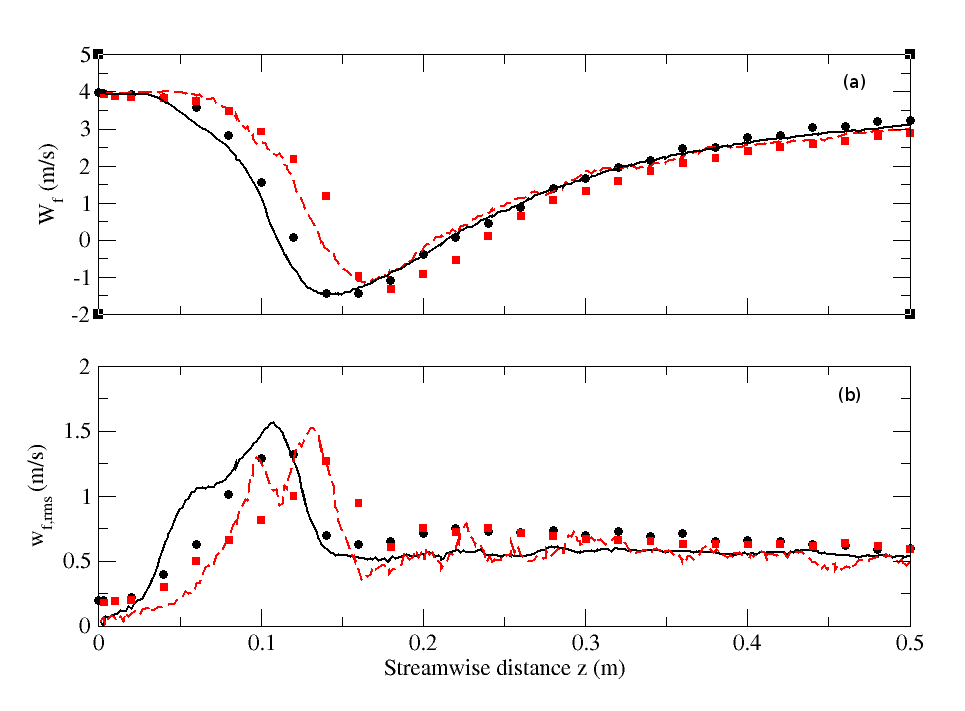
- The high mass loading case (M=110%) is more numerically challenging since the two-way coupling between the two-phases is expected to be strong. Figure (19) displays the axial profiles of mean streamwise velocity and turbulent kinetic energy for both single-phase calculations (M=0%) and two-phase calculations (M=110%). Numerical calculations are directly compared with measurements. It is clear that the presence of the dispersed phase at a high mass loading (M=110%) yielded a significant modification of the jet penetration and a total suppression of the recirculationzone as it is equally predicted by both experimental and numerical findings. The discrepancy between the physicaland the numerical experiments results is observed for the extent of the jet penetration whereas very good matching was obtained regarding the minimum value of the mean axial velocity as depicted by Fig. (19a).For the fluid RMS streamwise velocity, Fig. (19b) shows that differencesbetween the numerical and the experimental results are more significant in the zone (0.8m < z <0.16m) which is the same zone for which differences was also noticed between experimental and results regarding the mean axial velocity. In this narrow zone the turbulence intensity isunderestimated whereas the turbulence enhancement outside this zone was very well captured.
 | Figure 19. Streamwise profiles of (a) fluid mean streamwise velocity and (b) fluid RMS streamwise velocity for particle-free (M=0%) and particle-laden (M=110%) configurations. Circle: Experiment (M=0%); solid line: Numerical simulation (M=0%); Square: Experiment (M=110%); dashed line: Numerical simulation (M=110%) |
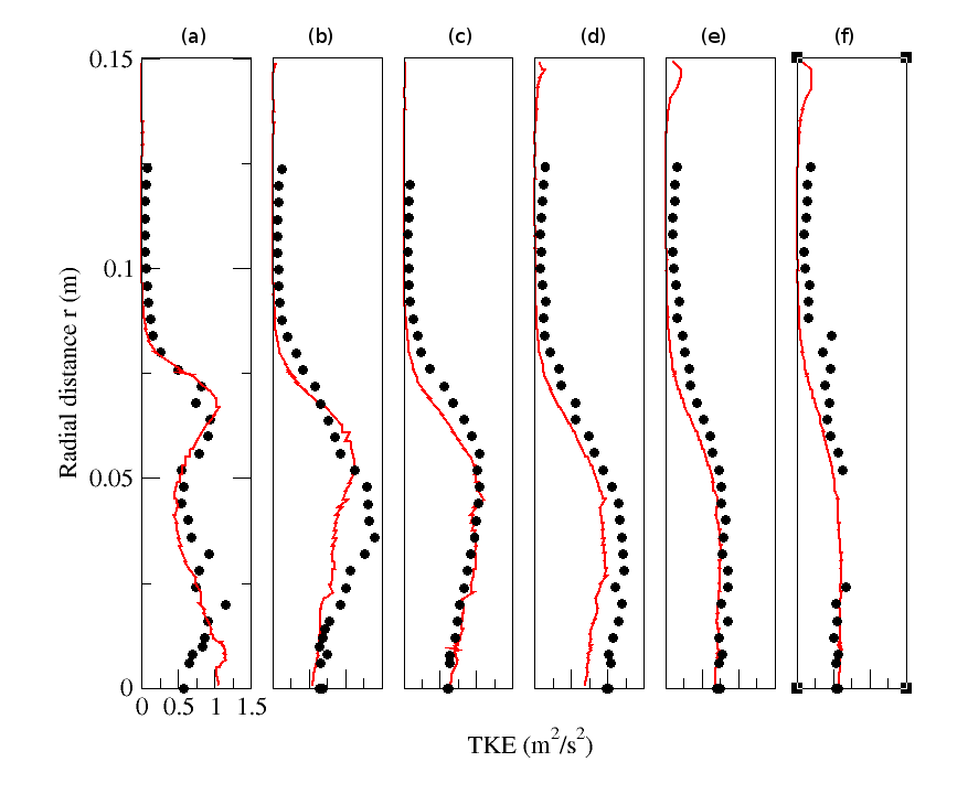
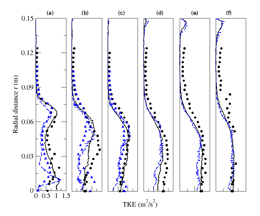 | Figure 20. Radial profiles of fluid turbulent kinetic energy. Circle: Experiment (M=0%); solid line: Numerical simulation (M=0%); Triangle: Experiment (M=110%); dashed line: Numerical simulation (M=110%). (a) z=0.08m; (b) z=0.16m; (c) z=0.20m; (d) z=0.24m; (e) z=0.32m ; (f) z=0.40m |
 | Figure 21. Radial profiles of fluid mean streamwise velocity for particle-free (M=0%) and particle-laden (M=110%) configurations. Circle: Experiment (M=0%); solid line: Numerical simulation (M=0%); Triangle: Experiment (M=110%); dashed line: Numerical simulation (M=110%). (a) z=0.08m; (b) z=0.16m; (c) z=0.20m; (d) z=0.24m; (e) z=0.32m ; (f) z=0.40m |
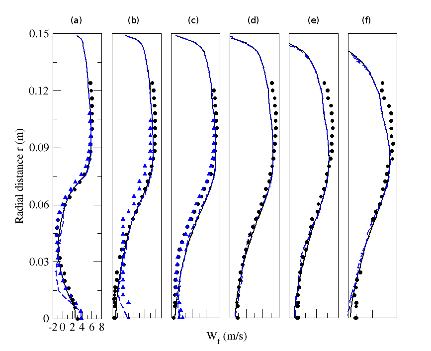
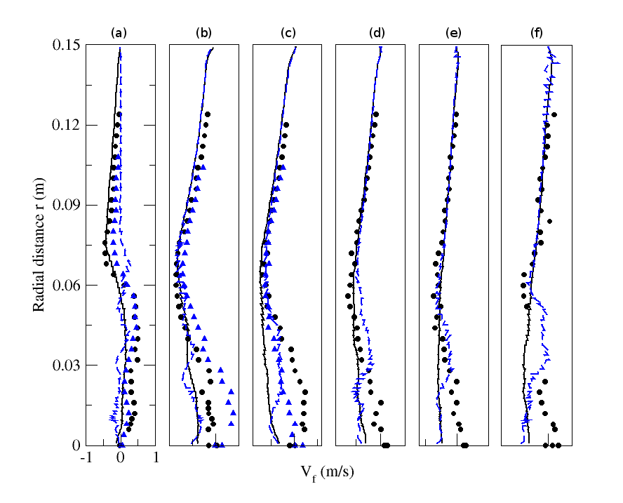 | Figure 22. Radial profiles of fluid mean radial velocity for particle-free (M=0%) and particle-laden (M=110%) configurations. Circle: Experiment (M=0%); solid line: Numerical simulation (M=0%); Triangle: Experiment (M=110%); dashed line: Numerical simulation (M=110%).(a) z=0.08m; (b) z=0.16m; (c) z=0.20m; (d) z=0.24m; (e) z=0.32m ; (f) z=0.40m |
4.2. Particle Phase
- Overall, Numerical predictions of the particle-phase mean and RMS velocities in both axial and radial directions are in good agreement with the experimental findings. As expected, the use of the stochastic LES model yields improved particulate results compared to results obtained using LES flow field (The latter are not shown here). Numerical results for the low mass-loading case (M=22%) show better agreement with measurements compared to the high mass loading case (M=110%). This is expected since the point-force scheme is known for its decreased performance for particle void fraction close to
 .It is worth to mention that in each control volume for the fluid phase, the different velocities of all the particles inside are mass-averaged following Fig. 4.
 4.2.1. Mass Loading: M=22%
- Figure (23) displays the streamwise profiles of mean, RMS axial and RMS radial particle velocities along the axis (R=0) for the low mass-loading case (M=22%). The results of the LES using the stochastic model are directly compared with measurements. Very good agreement between physical and numerical results is obtained except for the recirculation zone where minor discrepancies are noticed. In this criticalzone, particles decelerate, accumulate near the stagnation points, and stop before changing direction to escape from this zone by its sides. Thus, this zone is difficult to predict accurately for the particulate phase which explain the differences between the numerical results and the experiment.Radial profiles of the mean streamwise and mean radial particle velocities are depicted by Figs. (24) and (25) respectively at seven stations. Very good matching between the experimental and numerical results is noticed.
 | Figure 23. Streamwise profiles of particle (a) mean streamwise velocities, (b) RMS streamwise velocity, and (c) RMS radial velocity for particle-laden (M=22%) configuration. Circle: Experiment; solid line: Numerical simulation |
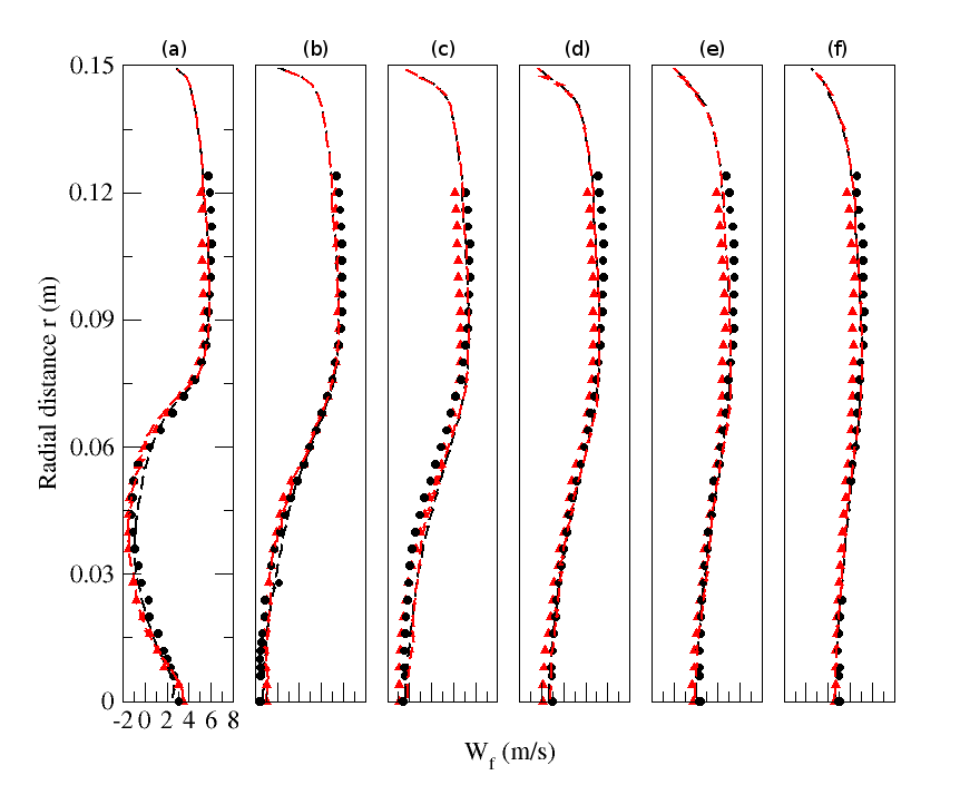
 | Figure 24. Radial profiles of particle mean streamwise velocity for particle-laden (M=22%) configuration. Circle: Experiment; solid line: Numerical simulation. (a) z=0.003m; (b) z=0.08m; (c) z=0.16m; (d) z=0.20m; (e) z=0.24m; (f) z=0.32m ; (g) z=0.40m |
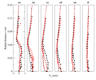
 | Figure 25. Radial profiles of particle mean radial velocity for particle-laden (M=22%) configuration. Circle: Experiment; solid line: Numerical simulation. (a) z=0.003m; (b) z=0.08m; (c) z=0.16m; (d) z=0.20m; (e) z=0.24m; (f) z=0.32m ; (g) z=0.40m |
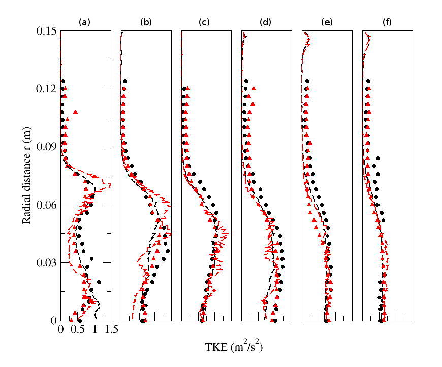
 | Figure 26. Radial profiles of particle RMS streamwise velocity for particle-laden (M=22%) configuration. Circle: Experiment; solid line: Numerical simulation. (a) z=0.003m; (b) z=0.08m; (c) z=0.16m; (d) z=0.20m; (e) z=0.24m; (f) z=0.32m ; (g) z=0.40m |
 | Figure 27. Radial profiles of particle RMS radial velocity for particle-laden (M=22%) configuration. Circle: Experiment; solid line: Numerical simulation. (a) z=0.003m; (b) z=0.08m; (c) z=0.16m; (d) z=0.20m; (e) z=0.24m; (f) z=0.32m ; (g) z=0.40m |
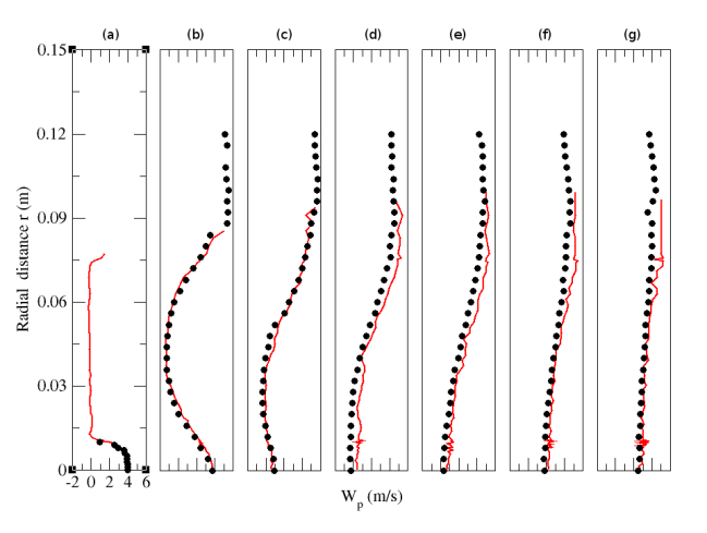
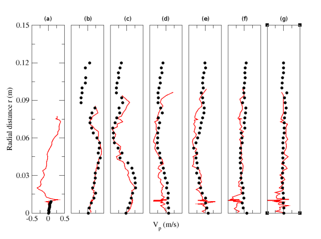
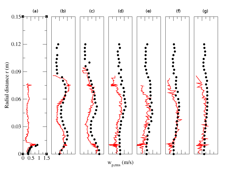
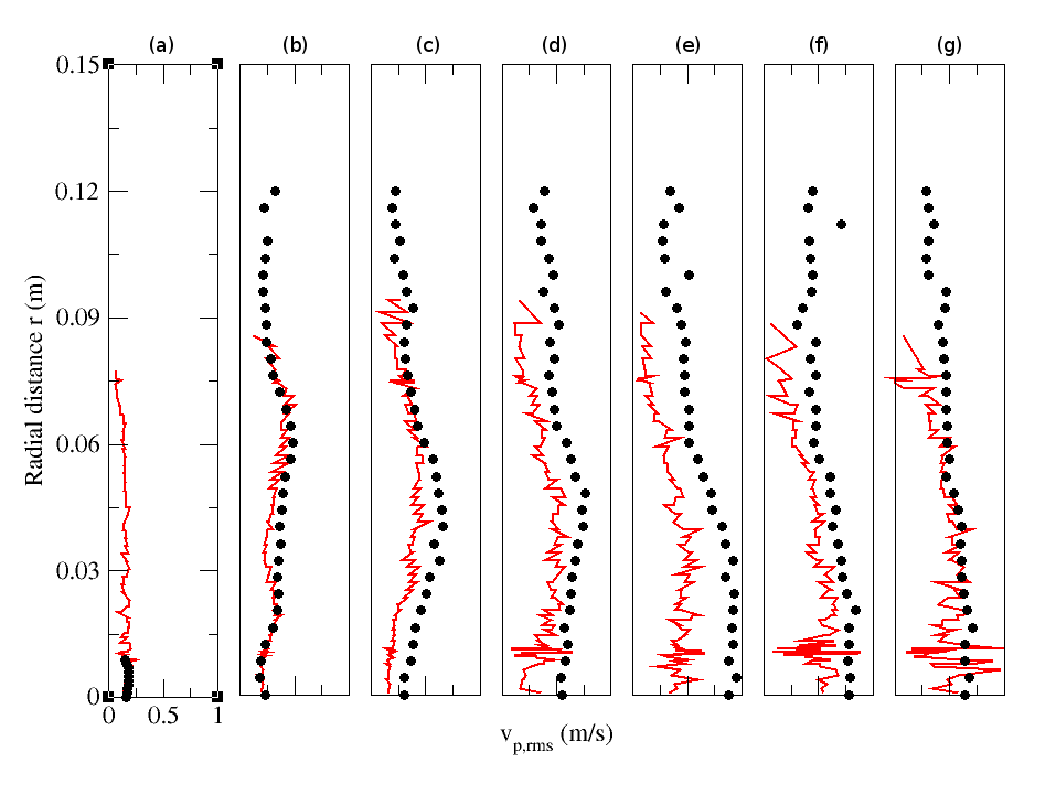
4.2.2. Mass loading: M=110%
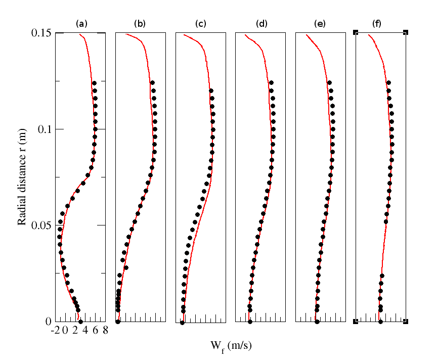
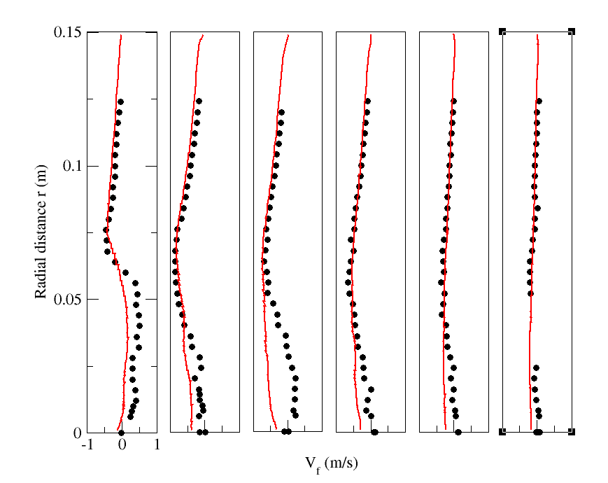
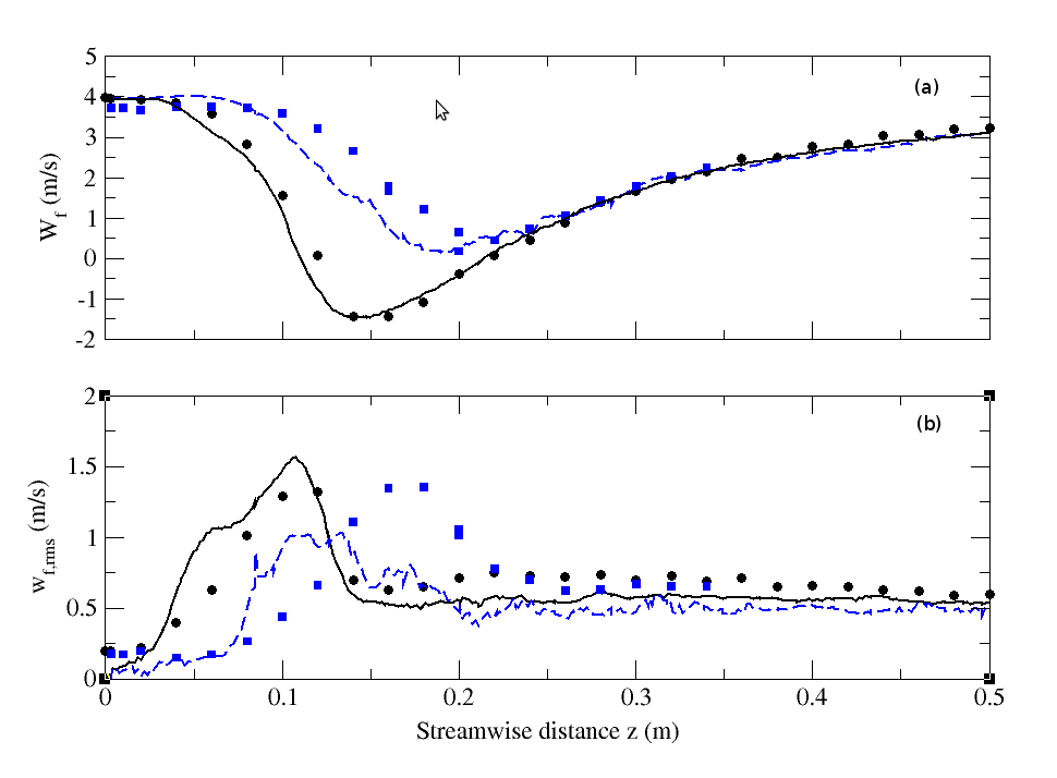
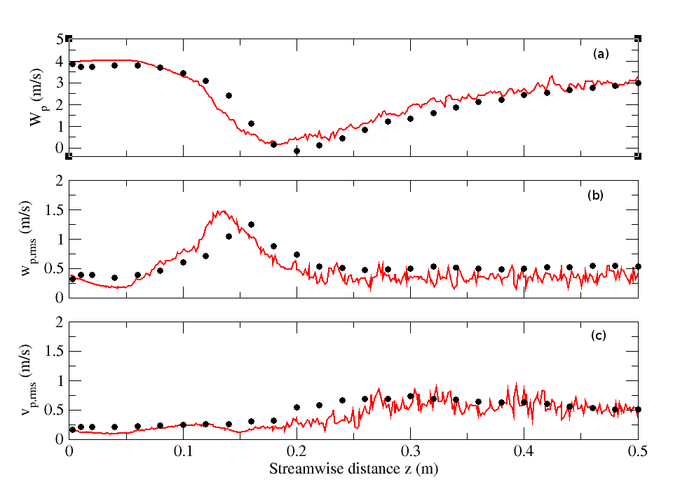
- Figure (28) displays the streamwise profiles of mean, RMS axial and RMS radial particle velocities along the axis (R=0) for the low mass-loading case (M=110%). The results of the LES using the stochastic model are directly compared with measurements. Very good agreement between physical and numerical results is obtained except for the RMS radial particle velocity downstream of z=0.15m
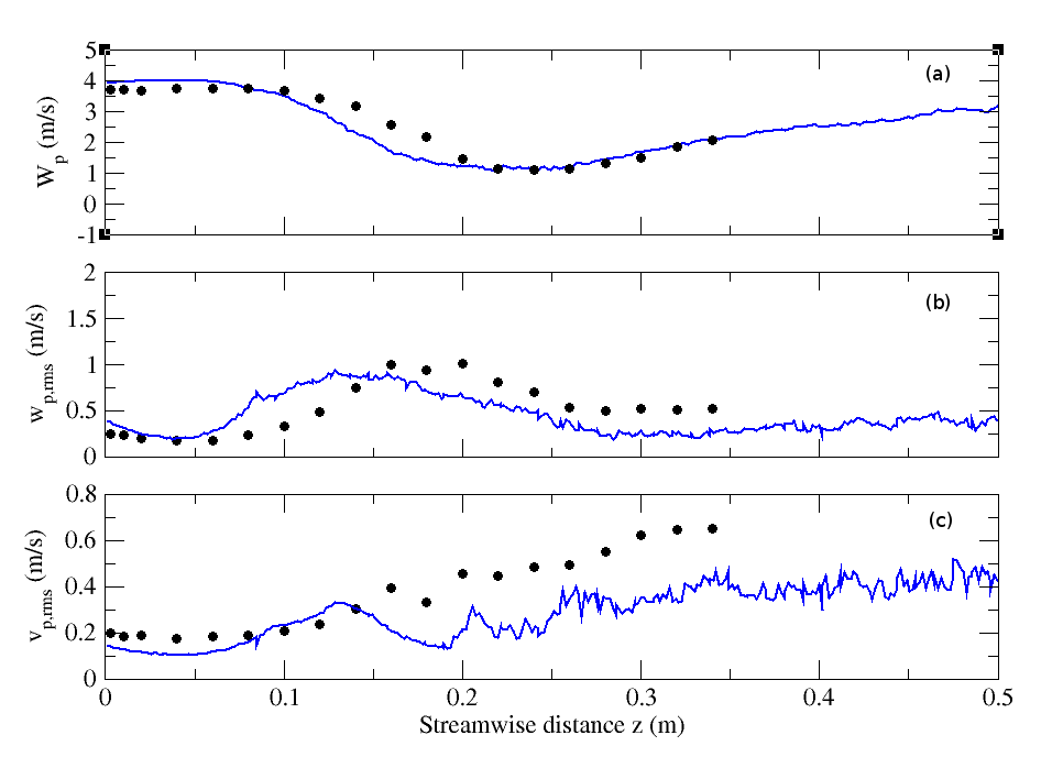 | Figure 28. Streamwise profiles of particle (a) mean streamwise velocities, (b) RMS streamwise velocity, and (c) RMS radial velocity for particle-laden (M=110%) configuration. Circle: Experiment; solid line: Numerical simulation |
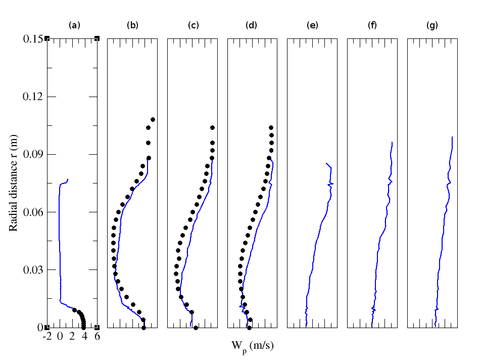 | Figure 29. Radial profiles of particle mean streamwise velocity for particle-laden (M=110%) configuration. Circle: Experiment; solid line: Numerical simulation. (a) z=0.003m; (b) z=0.08m; (c) z=0.16m; (d) z=0.20m; (e) z=0.24m; (f) z=0.32m ; (g) z=0.40m |
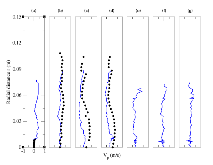 | Figure 30. Radial profiles of particle mean radial velocity for particle-laden (M=110%) configuration. Circle: Experiment; solid line: Numerical simulation. (a) z=0.003m; (b) z=0.08m; (c) z=0.16m; (d) z=0.20m; (e) z=0.24m; (f) z=0.32m ; (g) z=0.40m |
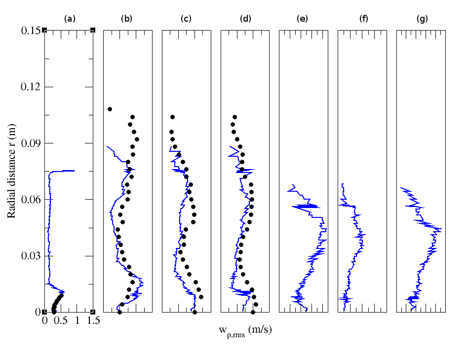 | Figure 31. Radial profiles of particle RMS streamwise velocity for particle-laden (M=110%) configuration. Circle: Experiment; solid line: Numerical simulation.(a) z=0.003m; (b) z=0.08m; (c) z=0.16m; (d) z=0.20m; (e) z=0.24m; (f) z=0.32m ; (g) z=0.40m |
 | Figure 32. Radial profiles of particle RMS radial velocity for particle-laden (M=110%) configuration. Circle: Experiment; solid line: Numerical simulation. (a) z=0.003m; (b) z=0.08m; (c) z=0.16m; (d) z=0.20m; (e) z=0.24m; (f) z=0.32m ; (g) z=0.40m |
5. Conclusions
- This work has presented the stochastic large eddy simulation approach to gas flow modification by solid particles. The bluff-body case studied experimentally by Borée et al.[27] was chosen as a validation case because it contains multiple complex flow features which are typical of combustion chambers.The point-force scheme was used to model the coupling between phases while Langevin-type diffusion process was deployed to account for the SGS turbulence discarded by filtering in LES calculations. The experimental findings show that for the high mass-loading case (M=110%), the turbulence is modulated by the particles to an extent that it suppressed the two stagnation points that were observed for the smaller mass loading case (M=22%)) and particle-free case.Furthermore, the existence of a recirculation zone where particles interact with negative axial fluid velocities constitutes a much more challenging test case for simulations compared to cases where the fluid and the particle mean velocities are of the same sign. This test case was an opportunity to assess the handling of two-way coupling situations in Code-Saturne and to see to what extent the stochastic model described earlier lends itself to LES of dispersed non-equilibrium turbulent shear flows in a two-way coupling situation.Numerical results on mean streamwisevelocities, mean radial velocities, and turbulent kinetic energy in radial and axial directions show very good agreement with the experimental findings. Some discrepancies were noticed, in particular for the high mass loading case (=110%). This is due to the limitation of the point-force scheme which should be replaced by a more accurate approach to the inter-phase coupling modeling in future works.
ACKNOWLEDGEMENTS
- Special thanks to EDF R&D for providing the open-source code: Code_Saturne and Professor D. Laurence from the University of Manchester, UK for his valuable comments on the manuscript.
References
| [1] | Crowe, C.T., Sommerfeld, M., and Tsuji, Y.: Multiphase flows with droplets and particles. New York, CRC Press Boca Raton FL, 1998 |
| [2] | Tsuji, Y., Morikawa, Y., Shiomi H., “LDV measurements of air-solids flow in a vertical pipe”, Journal of Fluid Mechanics, vol.139, pp. 417-434, 1984. |
| [3] | Rogers, C.B., Eaton, J.K., “The behavior of solid particles in a vertical turbulent boundary layer in air” International Journal of Multiphase Flow, vol.16, pp.819-834, 1990. |
| [4] | Kulick, J.D., Fessler, J.R., Eaton, J.K., “Particle response and turbulence modification in fully developed channel flow”, Journal of Fluid Mechanics, vol. 277, pp. 109-134, 1994. |
| [5] | Fessler, J.R., Eaton, J.K., “Turbulence modification by particles in a backward-facing step flow”. Journal of Fluid Mechanics, vol. 394, pp.97-117, 1999. |
| [6] | Crowe, C.T., “On models for turbulence modulation in fluid-particle flows”, International Journal of Multiphase Flow, vol. 26, pp.719-727, 2000. |
| [7] | Gore, R.A., Crowe, C.T., “The effect of particle size on modulating turbulent intensity”, International Journal of Multiphase Flow, vol.15, pp. 279-285, 1989. |
| [8] | Hosokawa, S., Tomiyama, A., “Turbulence modification in gas-liquid and solid-liquid dispersed two-phase pipe flows”, International Journal of Heat and Fluid Flow, vol. 25, pp. 489-498, 2004. |
| [9] | Hadinoto, K., Jones, E.N., Yuteri, C., Curtis, J.S., “Reynolds number dependence of gas-phase turbulence in gas-particle flows”, International Journal of Multiphase Flow , vol. 31, pp. 416-434, 2005. |
| [10] | Eaton, J.K., Segura, J.C., “On momentum coupling methods for calculation of turbulence attenuation in dilute particle-laden gas flows”, Mechanical Engineering Dept. Stanford University, Rep.TSD-135, 2005. |
| [11] | Squires, K.D., Eaton, J.K., “Particle response and turbulence modification in isotropic turbulence”, Physics of Fluids, vol.2, pp.1191-1203, 1990. |
| [12] | Sundaram, S., Collins, L.R., “A numerical study of the modulation of turbulence by Particles”, Journal of Fluid Mechanics., vol. 379, pp.105-143, 1999. |
| [13] | Lomholt, S., Stenum, B., Maxey, M.R., “Experimental verification of the force coupling method for particulate flows”, International Journal of Multiphase Flow, vol. 28, pp.225-246, 2002. |
| [14] | Crowe, C.T., Sharma, M.P., and Stock, D.E., “The particle-source-in cell (PSI-CELL) model for gas-droplet flows”, Transaction ASME. Journal of Fluid Engineering, vol.99, pp.325-332, 1977. |
| [15] | Segura, J.C., Oefelein, J.C., Eaton J.K., “Predictive capabilities of particle-laden large eddy simulation”. Mechanical Engineering Dept. Stanford University, Rep. TSD-156, 2004. |
| [16] | Paris, T., Eaton, J.K.,”Turbulence attenuation in a particle-laden channel flow”, Mechanical Engineering Dept. Stanford University, Rep.TSD-137, 2001. |
| [17] | Eaton, J. K., “Two-way coupled turbulence simulations of gas-particle flows using point-particle tracking”, International Journal of Multiphase Flow, vol.35, pp.792-800, 2009. |
| [18] | Balachandar, S., and Eaton, J. K., “Turbulent Dispersed Multiphase flow”, Annual Review of Fluid Mechanics, vol. 42, pp.11-133, 2010. |
| [19] | Elghobashi, S.E., “On predicting particle-laden turbulent flows”, Applied Science & Research, vol. 52, pp. 309-29, 1994. |
| [20] | Minier, J-P., Peirano, E., “The PDF approach to turbulent polydispersed two-phase flows”, Physics Reports, vol. 352, pp.1-214, 2001. |
| [21] | Boivin, M., Simonin, O., and Squires, K.D., “Direct numerical simulation of turbulence modulation by particles in isotropic turbulence”, Journal of Fluid Mechanics, vol.375, pp.235-263, 1998. |
| [22] | Squires, K.D., Eaton, J.K., “Effect of selective modification of turbulence on two-equation models for particle-laden turbulent flows”, Journal of Fluids Engineering, vol.116, pp. 778-784, 1994. |
| [23] | Elghobashi, S.E, Truesdell, G.C., “On the two-way interaction between homogeneous turbulence and dispersed solid particles. I: turbulence modification”, Physics of Fluids., vol. 5, pp.1790-1801, 1993. |
| [24] | Berrouk, A.S., Laurence, D., Riley, J.J., and Stock, D.E., “Stochastic modeling of inertial particle dispersion by subgrid motion for LES of high Reynolds number pipe flow”, Journal of Turbulence, vol.8, pp.1-20, 2007. |
| [25] | Berrouk, A.S., Stock, D.E., Laurence, D., and Riley, J.J., “Heavy particle dispersion from a point source in turbulent pipe”, International Journal of Multiphase flow, vol. 34, pp.916-923, 2008. |
| [26] | Berrouk, A.S., and Laurence, D., “Stochastic modeling of aerosol deposition for LES of 90 bend turbulent flow”, International Journal of Heat and Fluid Flow, vol. 29, pp.1010-1028, 2008. |
| [27] | Borée, J., Ishima, T., Flour, I., “The effect of mass loading and inter-particle collisions on the development of the polydispersed two-phase flow downstream of a confined bluff body”, Journal of Fluid Mechanics, vol.443, pp.129-165, 2001. |
| [28] | Riber, E., Moureau, V., García, M., Poinsot, T., Simonin O., “Evaluation of numerical strategies for large eddy simulation of particulate two-phase recirculating flows”, Journal of Computational Physics,vol. 228, pp.539-564, 2009. |
| [29] | Smagorinsky, J., “General circulation experiments with the primitive equations”, Monthly Weather Review, pp.91-99, 1963. |
| [30] | Germano, M., Piomelli, U., Moin, P., Cabot, W.H., “A dynamic sub-grid scale eddy viscosity model”, Physics of Fluids, A (3)7, 1991. |
| [31] | Lilly, D.K., “A proposed modification of the Germano sub-grid scale closure method”, Phys. Fluids, A (4)3, 1992. |
| [32] | Maxey, M.R., Riley, J.J., “Equation of motion for a small rigid sphere in a non-uniform flow”, Physics of Fluids, vol. 26, pp.883-889, 1983. |
| [33] | Kloeden, P.E., Platen, E.: Numerical solution of SDE through computer experiments. Springer-Verlag, New York, 1999 |
| [34] | Pozorski, J., Minier, J-P., “On the Lagrangian turbulent dispersion models based on the Langevin equation”, International Journal of Multiphase Flows, vol.24, pp.913-945, 1998. |
| [35] | Minier, J-P., Peirano, E., Chibbaro, S., “Weak first and second order numerical schemes for stochastic differential equations appearing in Lagrangian two-phase flow modeling”, Monte Carlo Methods Applications, vol.9, pp.93-133, 2003. |
| [36] | Wang, L.P., Stock, D.E, “Dispersion of heavy particles by turbulent motion”, Journal of Atmospheric Science, vol. 50, pp.1897-1913, 1993. |
| [37] | Sato, Y., Yamamoto, K., “Lagrangian measurement of fluid-particle motion in an isotropic turbulent field”, Journal of Fluid Mechanics, vol.175, pp183, 1987. |
| [38] | Heinz, S.: Statistical mechanics of turbulent flows. Springer-Verlag, Berlin. 2003 |
| [39] | Gicquel, L.Y.M., Givi, P., Jaberi, F.A., Pope, S.B., “Velocity filtered density function for large eddy simulation of turbulent flows”, Physics of Fluids, vol.14, pp.1196-1213, 2002. |
| [40] | Csanady, G.T., “Turbulent diffusion of heavy particles in the atmosphere”, Journal of Atmospheric Science, vol. 20, pp.201-208, 1963. |
| [41] | Minier, J-P., Peirano, E., Chibbaro, S., “PDF model based on Langevin equation for polydispersed two-phase flows applied to bluff-body gas-solid flow”, Physics of fluids, vol.16, pp.2419-2431, 2004. |
| [42] | Archambeau, F., Mechitoua, N., Sakiz, M., “Code_Saturne: A finite-volume code for the computation of turbulent compressible flows-industrial applications”, International Journal on finite volumes, vol.1, pp.1-62, 2004. |
| [43] | Laurence, D., “Large eddy simulation with unstructured finite volumes”, Direct and large eddy simulations VI. ERCOFTAC Series, vol.10, pp.27-38, 2006. |
| [44] | Celik, I.B., Cehreli, Z.N., Yavuz, I., “Index of quality for large-eddy simulations” In Proceedings of ASME FEDSM2003, 4th ASME JSME Joint Fluids Engineering Conference, Honolulu, Hawaii, 2003. |
| [45] | Pope, S.B., “Ten questions concerning the large-eddy simulation of turbulent flows”, New Journal of Physics, vol.6-35, pp.1-25, 2004. |
| [46] | Lain, S., Garcia, J.A., “Study of four-way coupling on turbulent particle-laden jet flows”, Chemical Engineering Journal, vol.61, pp.6775-6785, 2006. |