1. Introduction

In general, a permeable bed has recently treated analogously to an impermeable bed. The velocity distribution, and flow resistance coefficients were derived irrespective of bed porosity. However, significant interaction processes occur between the flow above and through the porous zone which depends on the permeability of the surface. These interactions influence a non–zero velocity at the permeable zone, and turbulence exchange of mass and momentum between the two flow zones. The exchange process is responsible for additional shear stress near the boundary[1].

Nowadays, several studies gave a sight on the velocity distribution within, and close to the porous zone, especially within the interface zone. Such as[2] published that the time- average stream-wise velocity increased much more near the free surface than near the permeable bed. It was found experimentally that the velocity profile over the suction zone consists of two parts; an inner boundary layer where the shear stress changes rapidly, and a logarithmic law is applied for the zone above the first layer in which the flow is unaffected by the presence of suction[3]. The logarithmic zone at the free stream has been widely applied such as[4-7].It was found that there is a significant increase in the near bed velocity and a velocity reduction near the water surface, resulting in the formation of uniform velocity distribution[2].

Although, the vertical velocity distribution is an important variable to be studied and analyzed as it gives a good indication about the fluid movement in the interface region, the previous studies focus on the longitudinal velocity as most of it deals with the free stream, where no vertical velocity exist.

Fully developed turbulent flow through and over permeable bed is characterized by the momentum transfer occurring from the faster flow at the free stream and the slower flow in the porous zone. This phenomenon occurs at the interface zone, where a shear layer develops. It is developed with the secondary currents generated at the corner regions of the cross section, bed-generated turbulence, and free surface effects. These phenomena result in a very complicated flow field that studied by lots such as;[5] and[8- 10].

(1)

It was shown in that turbulence can penetrate into the pore space between the obstacles. The interface zone can therefore be defined as the region of the porous medium and free stream influenced by the free stream flow. The thickness of the interface zone is called the penetration width.

A dynamic relationship between the roughness layer thickness and (C_dα)^-1 using data from different obstructed flows, and found that δ_v = 0.333(C_dα)^-1[12]. This indicates that the extent to which transport length scale of the thickness (C_dα)^-1 determines the vertical transport length scale δ_v.

Turbulence is three-dimensional time dependent non-linear phenomenon. The main characteristic of turbulence is the transfer of energy from larger to smaller length scales. Large energy from the mean flow is extracted by the large eddies and then transferred to neighbouring eddies of smaller scale. The smallest eddies then lose energy through the action of viscous dissipation rate, which finally convert into thermal energy.

Turbulence can be described by several variables, such as, the turbulent kinetic energy, and turbulent dissipation rate. The turbulent kinetic energy is characterized by root-mean –square of velocity fluctuations. Due to the difference between velocities in the free stream and porous zone, the turbulence increases at the interface zone.

Several studies published about turbulent kinetic energy within and over permeable beds such as[10]. The effect of suction rate on TKE was studied by[15] and found that decreasing the suction rate up to 9% decreases the TKE more than four times.[16] found that within the range of Reynolds number of their analysis, the penetration of the turbulence remains independent of the Reynolds number. Further, the existence of an extra production term in the TKE-equation is important in the porous region.

Still lots of detailed analysis needed in order to overcome all the factors that affect the turbulent flow within and over permeable bed such as the effect of flow geometries, and or the effect of the density of the porous zone. Further, literature contains lots of studies about the flow features and factors affecting them. However, because of the complexity of the system within the free stream and the porous zones, up to the author’s knowledge there is a leakage of knowledge at this area of study. Further, few studies in this area used spatially averaged technique to overcome flow heterogeneity due to both turbulence and presence of solid obstacles.

The main objective of this paper is to study the characteristics of the mean flow and turbulence within and over a permeable bed in detail. The whole flow domain can be divided into the three important flow zones: free stream, porous layer, and the interface between them. The simulation results include mean velocities and various turbulence quantities (turbulent kinetic energy (TKE), turbulent shear stress, TKE production and dissipation).

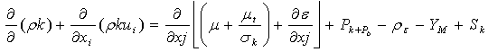
2. Governing Equation

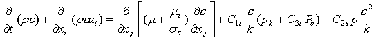
In general, two equation models are widely used in present engineering calculations to solve Reynolds Averaged Navier Stokes (RANS) equation. It gives independent scales (eliminates the need for specifying the turbulence length scale) in calculating the turbulent viscosity (μ_t). The numerical solution for the 2-D model used in this study is K-epsilon. Within the K- epsilon model there are a three solution models available Standard, RNG, and Releasable models. The solution in this study is by two equation model using k-epsilon (k-) model which is widely used in literature.

The two equations solved in K- epsilon model are the turbulent kinetic energy, and the turbulent dissipation rate:

(2)

The dissipation :

(3)

where :

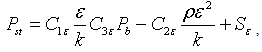and P_st =0.0 at RNG model , for RNG model, and P_RNG = 0.0 at standard model Coefficients _k, , C₁, and C₂, are empirical constants. The turbulent viscosity (_t) is[], and P_k represent the generation of turbulence kinetic energy due to the mean velocity gradients , P_b represent the generation of turbulence due to buoyancy, , and eddy viscosity is computed by . It should be mentioned here that the strain rate (S) in both equations is, where, the strain rate tensor and the degree to which ε is affected by the buoyancy is determined by the constant C_{3 ε} which equals

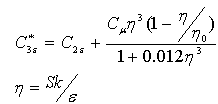In the present study, the commercial CFD software Ansys- Fluent is used. In common with many other codes, Fluent solves the Navier Stokes equation numerically using the finite volume method on an unstructured grid. The Navier stokes equations consist of a continuity and three momentum equations, which are based on the conservation of mass and momentum respectively ([17]).

3. The Simulated Cases

The study was a numerical simulation for fully developed turbulent flow zone over and through permeable bed. The data for all simulated cases are defined in[18]. They carried out their experimental and numerical study for three different bed porosities. These cases involved turbulent flow over and within three and four layers of rods. These rods were fixed at different distances to enable to include the porosity effect on turbulence. Reference[18] computed the flow structure above and within the porous medium using a model based on the Reynolds – averaged Navier-Stokes equations. It was solved using Fluent software with the k-epsilon method. In their simulation, a periodic boundary condition was used. The periodic boundary conditions may do not accurate results within the porous zone as the flow passes around the rods from vortices the may be cut before it is complete and the flow pattern before and after the rod is not the same which is the basic in periodic boundary condition computation. In this study long flume is built for the studied cases. This enables us to reach fully developed turbulent flow in conditions as the real experiments.

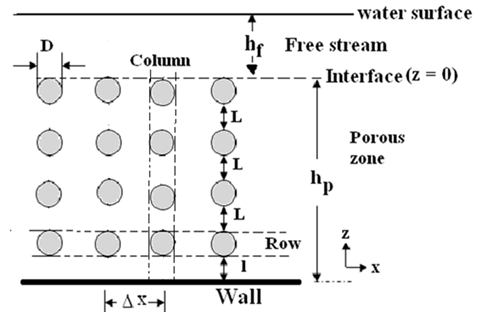Figure 1. Columns of the arranged rods bundle and symbols for geometry

Table 1. Geometric and Hydrodynamic Characteristics Case dens30 dens50 spar30 spar50 spar70 D (mm) 11.5 11.5 10 10 10 ∆x(mm) 13.5 13.5 25 25 25 hf (mm) 30 50 30 50 70 L(mm) 2.5 2.5 10 10 10 l (mm) 1.5 1.5 5 5 5 Nrod/column 4 4 3 3 3 Rno 6.1x103 1.479x104 4.918x103 1.211x104 2.201x104 Porosity 0.440 0.440 0.8126 0.8126 0.8126

The geometries of the cases were built in Gambit software. The permeable bed was consisting of a bundle of rods mounted at certain locations at the bottom of the bed. The water flows over and through these rods. Five different cases were selected with the geometries shown in Table (1). Figure (1) shows the arrangement of rods bundle.

Then it is exported to Ansys12 (Fluent) for simulation. A sensitivity analysis has been done for spar30 case, as it can be computed with larger mesh size, and as the computation time in Fluent is large, and the expected accuracy will be less for larger mesh. Therefore, the dense cases have not been mesh tested. To test the mesh size affect on the solution. Case spar30 was meshed three times, each with different mesh sizes. The mesh for all cases studied was triangular. Each case having nearly a double mesh size of the previous smaller one, with 0.45 mm for the smallest size. The testing was for the results that show mesh independence. The results show that the mesh size of 0.98 and 0.45 mm leads to the same results. For this the mesh size of 0.98mm was selected for the spars cases. The exported cases from Gambit are used in simulation in Ansys12 (Fluent) software, with the flowing boundary condition, and solution controlled methods:

The numerical model selected was k – ε with one of the two models mentioned at section. Under the solution methods the pressure-velocity coupling scheme option selected is “Simplec” with skewness correction of 2. Simplec scheme improves convergence for pressure-velocity coupling[19]. The spatial discretization selected are; the gradient is ”Least Square cell Based”, the pressure, momentum, turbulent kinetic energy, and turbulent dissipation rate are all ”Second Order Upwind”.

Under the solution methods the pressure-velocity coupling scheme option selected is “Simplec” with skewness correction of 2. Simplec scheme improves convergence for pressure – velocity coupling (Fluent user Guide, Chapter 18 in www.Fluentusers.com). The spatial discretization selected are; the gradient is ”Least Square cell Based”, the pressure, momentum, turbulent kinetic energy, and turbulent dissipation rate are all ”Second Order Upwind”. The appropriate boundary conditions for the present problems are set as a uniform flow at the entrance with inlet velocity, a no slip condition at the impermeable wall, symmetry at the free stream region, outlet pressure at the exit. The interior edges identified as interior zone in the simulation. The simulation was consumed a long time and large number of iterations to reach fully developed turbulent flow shown in Table 2. The fully turbulent flow is the zone were the flow features do not change with distance. In this study it was tested at each 100 mm distance for more than five different x-locations.

3.1. Model Testing and Validation

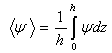
In this study, the values of various flow parameters are kept the similar to that published[18] to assure correctness and consistency of the simulated results. The results simulated were tested for their validation[18]. Further, two simulated results from spars cases were tested with[16] who simulated these results using macroscopic technique to solve the (RANS) equations. Figure 2 shows a comparison between published and present data for normalized turbulent kinetic energy (TKE⁺) vs. normalized bed height for a mid-line between two column rods. From the figure, it can be concluded that the simulation is with reasonable results that is superior closer to experimental results than previous studies at the interface between the free stream and the porous zone.

Table 2. The Geometries of The Simulated Cases Case L/D Face mesh Size, mm(free stream) Face mesh Size, mm (porous zone) Selected Model No. of iterations spar30 57 0.98 0.98 RNG 121880 spar50 48 0.98 0.98 Standard 836110 spar70 43 0.98 0.98 Standard 943640 dens30 38 0.9 0.5 Standard 1647115 dens50 32 0.9 0.5 Standard 2022740

4. Results and Discussion

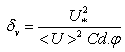
The work described here was undertaken to provide more detailed information about the velocity field and turbulence within the fully developed turbulent region. The data that exported from Fluent was irregular. Further, it was heterogeneous. To overcome these problems, a Matlab program was built for each case to convert the data to regular and to spatially averaged to overcome the flow heterogeneity. Spatial averaging was for conventional bed-parallel volumes (centre to centre column rod) for obtaining vertical properties of velocity components. The spatially averaged quantity of a flow variable ψ is defined as:

(4)

Where: h is the flow zone thickness.

4.1. The Velocity within and Over the Permeable Bed

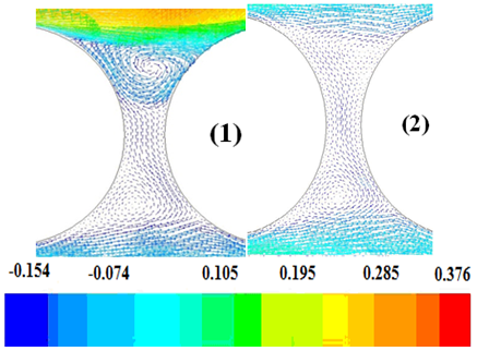
The flow velocity through and over the porous zone is shown as contours at figure 3. This figure is for longitudinal velocity for two different porosity cases. From the figure, it could be noticed that the overall flow pattern is similar for both shown cases.

The mean velocities show the expected boundary-layer profile in the free stream zone, and a much slower flow in the porous zone. A pipe-like velocity profile forms between each two successive rows of cylinders, with a faster and more developed flow in case of sparse cylinder packing, compared to the dense case. CFD provides details of the flow spatial structure between the cylinders, where the difference between the sparse and the dense packing is most pronounced. As expected bed porosity has a major influence on the flow velocities within the porous layer.

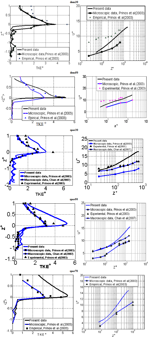Figure 2. Comparison Between Previously Published and Present Study for Normalized Turbulent Kinetic Energy Profile Above and Within Porous Medium(Left), and Normalized Velocity Distribution at The Free Stream(Right) for The Simulated Cases

The longitudinal flow velocities across the overall flow profile including both free stream and porous zone are shown in Figure 3. For comparison, each Figure shows the results for the ‘sparse’ case (top) and ‘dense’ case (bottom). The overall flow pattern for both cases are similar: as expected, velocity magnitudes are much larger in the free stream than within the porous zone; furthermore, within the free stream, the velocity profile has the shape typical for the boundary layer flows, whereas within the porous zone velocity profile is similar to the pipe flow. The ‘pipes’ within the porous zone for ‘sparse’ and ‘dense’ case are very different: in the former case they have much bigger diameter, which penetrates into the horizontal gap between the two adjacent rods; in the latter case the ‘pipe’ is very narrow and it maintains practically constant diameter. The ‘sparse’ case shows another interesting feature – the maximum flow velocity in the highest pore is somewhat smaller than in the second pore. This is in agreement with the experimental results of Pokrajac et al.[20], who provide a detailed discussion of the physical mechanisms behind this counterintuitive result.

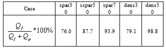
From the profiles of the longitudinal velocity (Figure 3) it is clear that majority of flow occurs in the free stream zone. The percentage of the total discharge flowing through free stream zone is computed as: (), where: Q_f, and Q_p are the volumetric flow rate within the free stream and the porous zone, respectively. The results are shown in Table 3. From the table it can be concluded that a large discharge difference exists between the porous and free stream zones, even when the area of flow is smaller than that at the porous zone. Further, as expected a comparison between the studied cases shows that the discharge difference between the free stream, and the porous zone, increases with the density of the rod packing. Furthermore, the larger is the free stream thickness, the larger is the discharge difference. This result is in agreement with experimental results of[21].

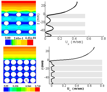Figure 3. The Longitudinal velocity distribution (m/s): Contours (Left) and the profile along the central line between two-rod columns (Right), for spar30 Case (Top) and dens30 Case (Bottom). Grey Areas on The Right Indicate The Position of The Rods

Table 3. The Discharge Within the Free Stream, Relative to the Total Discharge

In more detail, Figure 4, and 5 show the flow vectors coloured by longitudinal velocity for both spar30, and dens30 cases. The flow area over, and underneath the rods are smaller than between two column regions. This decrease in the cross sectional area, increases the velocity. Beyond this region, the cross sectional area increases, so the flow velocity decreases. This pattern obeys fluid dynamics laws “velocity is inversely proportional to flow cross sectional area”. At spar30 case, there is sufficient distance for the vortices to form two complete vortices behind the rod and then the flow return back before it reaches the second rod. However, the scenario within the dense cases is different, as due to the small distances between the rods the flow is nearly stagnant in between the rods. As there is no sufficient spaces, the vortices forms at the upper and lower regions of the rods at the centre side between each two-column rods. In this study, it is noticed that within the interface zone, the velocity is with wave patterns. These waves can be seen at the contour plots in Figure 3. This is due to the high flow difference between free stream and the upper part of the obstacle, where there the velocity is nearly zero.

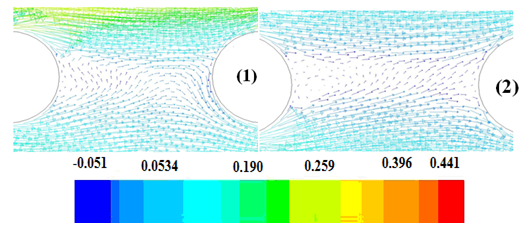Figure 4. The velocity vectors between two adjacent rods for spar30 (left), and dens30 (right) cases; rods are numbered top-down. Vectors are colour-coded based on Ux

Figure 5. The Velocity vectors between two adjacent rods for top rod (left), and second rod (Right) at dens30 ; vectors are colour-coded based on lateral velocity

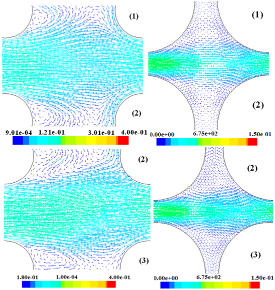Figure 6. Velocity vectors (m/s) in the free space between The rods; spar30 (Left), and dens30 (Right) cases; rods are numbered top-down. vectors are colour-coded based on lateral velocity

Velocity vectors are shown in Figure 6, this time highlighting flow within the longitudinal pores in the gap between the adjacent rows of the rod. Velocity magnitudes in the pore are smaller than in the second pore for both sparse and dense case. In the former case, the geometry of the two pores is also different, especially in the upper part. As stated earlier, this is the effect of the surface flow which penetrates between rods and changes the geometry of the flow in the first pore.

In closer insight, for the flow features (velocities, and turbulence) were averaged in a Matlab program. The longitudinal velocity within the bed varies from zero close to the solid surface to the highest at the med point between two rows of rods. Figure 7 shows a comparison between the spare and dense cases for normalized longitudinal velocity distribution within the porous zone. Both cases were normalized (dimensionless) to overcome the geometry difference between both cases. The velocity was normalized by dividing it by shear velocity (U/U_*). The vertical distance within the porous zone was made dimensionless, using[h*_rod = (z + d/2)/h_rod -1], where h_rod is the rod centre to centre vertical distance in order to align the vertical position of the rods in the dense and sparse cases. This gives the position of rods 1, 2, 3 as h^*_rod = -1, -2, -3, respectively. From figure 7, and 8, it can be noticed that as the porosity increases, the bed longitudinal velocity, also increases. Further, for the sparse case, the velocity is small but still positive in the region between the two columns. On the other hand, the dense case shows a stagnant flow close to the rods, that reaches negative values at the upper part of the top rod.

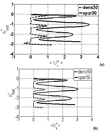Figure 7. Normalized longitudinal velocity within the porous zone Porosity effect on normalized longitudinal velocity for flow within porous zone; (a) for spars cases, and (b) dense cases

The free stream thickness affects the flow within the porous zone porous zone. Figure 9 shows the effect of free stream thickness on velocity within porous zone, a, and b longitudinal velocity for spars, and dens cases respectively, and c is for vertical velocity. From the figure, it can be concluded that the higher the free stream water thickness the lower flow velocity within the porous zone.

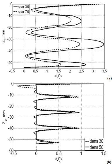Figure 8. Free stream thickness effect on the longitudinal velocity within the porous zone; (a) for spars cases, and (b) dense cases

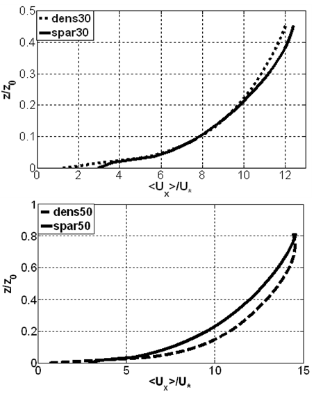Figure 9. Effect of bed porosity on the longitudinal velocity in the free stream zone

Figure 10 shows a contour plot for the vertical velocity distribution, and the vertical velocity distribution along the central line between two column rods. From the figure it can be seen that within the porous zone, the velocity changes from negative to positive at different parts of the porous bed with a highest value at the interface zone. This feature is due to the change in flow direction because of presence of rods. At the interface zone, the flow passing over the upper rod meets with the high speed at the free stream. Both the differences in speed and flow direction between the upper and lower zones of the bed increase the turbulence generation at the interface zone. However, at the free stream the vertical flow decreases to reach zero as the flow changes to a longitudinally uniform flow.

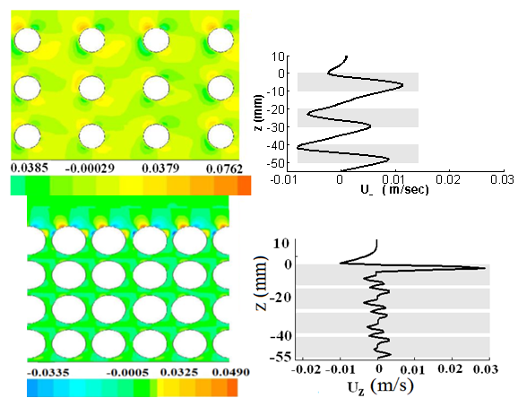Figure 10. The bed-normal velocity distribution (m/s); contours (left) and the profile along the central line between two rod columns (right), for spar30 case (top) and dens30 case (bottom).Grey areas on the right indicate the position of the rods

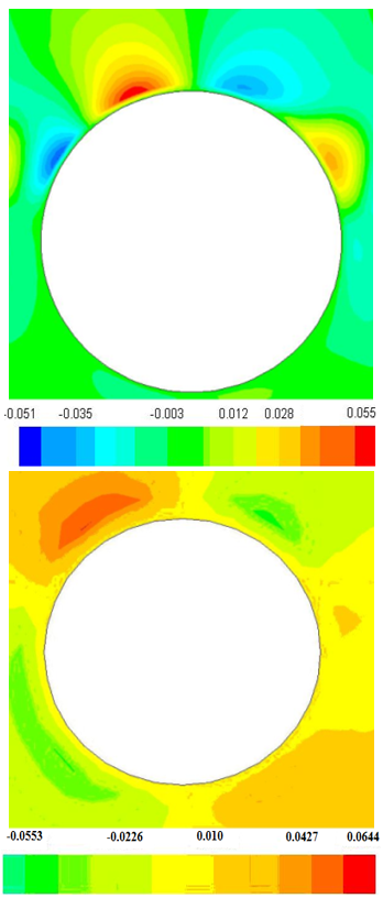Figure 11. The Vertical Velocity Contours Around a Top Rods; dens30 (UP) and spar30 (Bottom) Cases

Figure 11 shows the vertical velocity contours, and distribution with the flow stream for the top rod. From the figure it can be estimated that the spar30 case showed within the porous zone the vertical velocity is fluctuating. It is changing around the rod. It has a high value at the upper inflow, and at the lower outflow side of the rod. The high values are due to the change of flow direction because of the presence of the obstacle.

The penetration width (roughness layer thickness) has been previously studied in several publications such as[22] who suggested that the penetration width is defined as the distance from the surface of the porous zone to the point where shear stress decays to 10% of its maximum value. Applying this proposition at the simulated cases resulted penetration thickness values shown in Table 4. From the table it can be concluded that the larger the porosity the lower the penetration width. This gives indication that the transient layer between the free stream (fully developed turbulence), and the porous zone is affected with the free stream thickness. This result is very important for environmental engineering studies at open channels for pollutant migration from flow zone to another.

The dimensionless (δ_v/d) is plotted against scale parameter (C_dαd)^-1 in Figure 12. Where C_d is the drag coefficient, is the frontal area per unit volume, computed for the top rod. From the results it can be concluded that the larger the porosity the larger the penetration width. These results agree with the experimental results of[22-24]. Further, the higher the free stream thickness showed a larger penetration layer thickness, which disagree[8].

Table 4. Penetration width at the interface

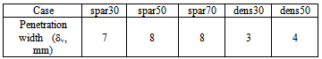
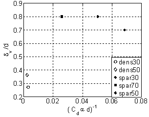Figure 12. Penetration thickness, versus (Cdαd)-1

4.2. Turbulence within and Over the Permeable Bed

Figure 13 shows the contour plots and vertical profiles of TKE for sparse and a dense case. For both cases, TKE has a clearly defined maximum close to the interface. This is due to the difference between velocities in the free stream and porous zone, which creates the most intense shearing at the interface. Within the free stream, TKE decreases with distance from the bed. Overall, the TKE pattern agrees with different published data such as;[16] and[18]

Turbulence within the porous zone is heterogeneous and characterized with very small values of TKE. For the sparse case, TKE within the porous layer steadily increases towards the interface. However, the dense case has higher TKE values close to the interface where TKE reaches maximum. In this region, the TKE value for the dense case is nearly double that of the sparse case. This is probably due to the higher difference in velocity between the free stream, and the porous zone, which enhances shearing and hence also generation of turbulence.

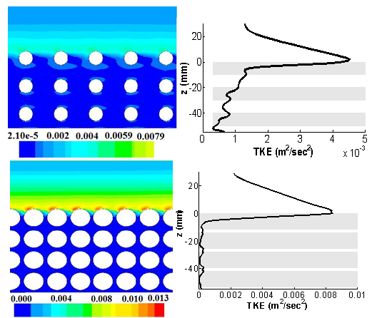Figure 13. The turbulent kinetic energy distribution (m2/s2): contours (left) and the profile along the central line between two rod columns (right), for spar30 case (top) and dens30 case (bottom). Grey zones on the right indicate the positions of rods

Figure 14 shows normalized spatially averaged TKE distribution[]; within the free stream (top), and within the porous zone (bottom) for both flow depths the sparse case has higher TKE in both free stream and porous zone compared with the dense case. Further, higher free stream thickness shows a higher TKE. Overall, the TKE profiles in the porous zone show a distinct difference between the sparse case, where turbulence penetrates vey deep into the bed and the dense case where does not go beyond the centre of the top rod.

The turbulent energy production (TKEP) was normalized by dividing the spatially averaged TKEP with ρ.U_*² (Figure 15). From the figures it can be concluded that a larger TKEP rate in the dense case compared with the sparse. Further, the larger free stream thickness, have a larger TKEP.

The turbulent dissipation rate (TDR) is the rate at which the turbulent energy is absorbed by breaking the eddies down into smaller until it is ultimately converted into heat by viscous forces. Figure 16 shows the normalized averaged turbulent dissipation rate over the free stream and the porous zone. From the figure, it can be concluded that TDR is lower when free stream thickness is higher, and the porosity effect is smaller than the effect of free stream thickness.

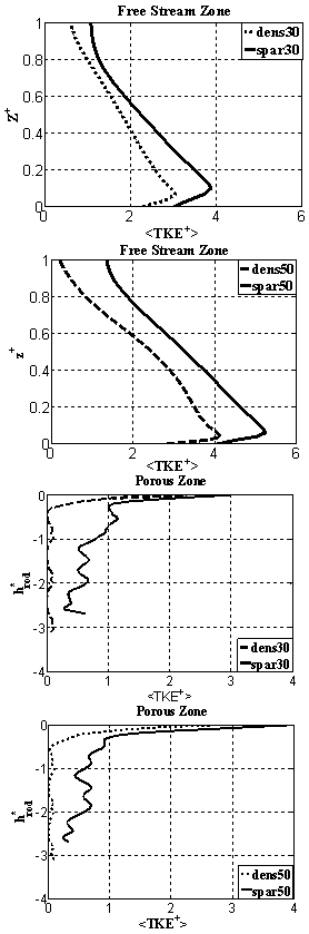Figure 14. Normalized spatially averaged turbulent kinetic energy distribution with normalized bed height at both free stream zone (Top), and porous zone. Bed normalized coordinate is (z/hf)

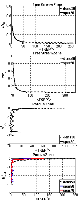Figure 15. Normalized turbulent kinetic energy production distribution at both free stream zone (top), and porous zone (bottom) for different studied cases

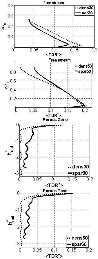Figure 16. Porosity effect on the turbulent dissipation rate in both free stream (Top) and porous (Bottom) regions

5. Conclusions

A detailed analysis was made to some flow variables to increase our understanding of turbulent flow through and over permeable bed. These variables were the vertical and longitudinal velocities, turbulent kinetic energy, turbulent dissipation rate, and the energy consumed by flow. The study covers free stream, porous and interface zones. Further, the porosity effect and the free stream thickness were also included in the simulation. The following results were gained from the analysis.

• Mean velocities show the expected boundary-layer profile in the free stream zone, and a much slower flow in the porous zone. A pipe-like velocity profile forms between each two successive rows of cylinders. As expected bed porosity has a major influence on the flow velocities within the porous layer.

• TKE in the free stream region have the expected shape with a maximum value close to the wall and the minimum close to the free surface. Within the porous layer there is a clear difference between the sparse and the dense arrangement: in the former case TKE penetrates practically throughout the whole porous layer, whereas in the latter case it penetrates only until the half of the top layer of cylinders.

• TKE production and dissipation rate show very similar features. Turbulent shear stress in the free stream shows the expected approximately linear profile. Within the porous layer, the sparse case has a linear shear stress profile alternating between positive and negative values, typical for a pipe flow, whereas for the dense case the shear stress within the porous layer is practically zero.

ACKNOWLEDGEMENTS

The writer gratefully acknowledge Dr Dubravaka Pokrajac for her writing comments.