-
Paper Information
- Next Paper
- Previous Paper
- Paper Submission
-
Journal Information
- About This Journal
- Editorial Board
- Current Issue
- Archive
- Author Guidelines
- Contact Us
American Journal of Fluid Dynamics
2012; 2(4): 42-54
doi: 10.5923/j.ajfd.20120204.03
Sound Scattering Laws for Moving Microinhomogeneous Media
 Abstract
 Reference
 Full-Text PDF
 Full-Text HTML
Andrew G. Semenov
Acad. N.N. Andreev’s Acoustics Institute RAS, 4 Shvernik street, Moscow, 117036 Russia
Correspondence to: Andrew G. Semenov , Acad. N.N. Andreev’s Acoustics Institute RAS, 4 Shvernik street, Moscow, 117036 Russia.
| Email: |  |
Copyright © 2012 Scientific & Academic Publishing. All Rights Reserved.
Low frequency sound scattering in microinhomogeneneous media, comprising particles moving orderly or chaotically with respect to ambient ideal or viscose fluid or streamlined by fluid is analyzed. It is shown that basic scattering laws are violated in moving media due to acoustic / electromagnetic wave scattering analogy violation related to ambient fluid entrapment by particles (inhomogeneities) playing noticeable role in media sound scattering. Moving inhomogeneous media low frequency sound scattering data observable in experiments is frequently distinguished from predicted by sound scattering theory. That is why scattering laws in moving media are to be generalized and it is main purpose of the paper. Scattering amplitudes and crossections for ideal potential and viscose flows generated by particles moving with respect to media are calculated by means of inhomogeneous wave (Lighthill’s) equation. For spherical scatterers in orderly motion Rayleigh law acquires correction in particle Mach number linear approximation even in ideal fluid. However, for chaotically moving particles in ideal fluid, it still holds on the average. Reynolds number of particles motion, angle of scattered wave incidence and flow Mach number – incident wave parameter relationship, defines more complex sound scattering law versions valid in viscous media distinguished from classical Rayleigh law. Linearity of Lighthill’s equation (low Mach number requirement) is analysis restriction. PACS numbers: 43.20.Fn, 43.28.Gq, 43.28.Py
Keywords: Microinhomogeneneous Media, Sound Scattering, Orderly or Chaotically Moving Particle, Movable Particle, Attenuation Law, Ideal and Viscose Flow, Reynolds Number
Article Outline
1. Introduction
- The phenomenon of wave scattering in inhomogeneous medium is our surrounding world notion basis. Although Tyndall and Rayleigh as far back as formulated its general concepts in the 19th century, various aspects of it still attract scientists’ efforts[1-22]. They are pretending to explain observable experimental data (wave attenuation laws) by simple theoretical model or concept, say, by original Rayleigh law[1, 14], by statistical properties of media frozen turbulence[4, 7, 8-13] leading to Rayleigh law as well or even by supposed underwater sound field fractal nature[15]. Weakness of first model observed for moving media will be discussed below. In fact, major part of paper is devoted to its correction. The problem of second model (concept) lies in discrepancies observed experimentally in low frequency sound scattering limit. Even if sound absorption is negligible, attenuation law frequency dependence in infrasonic limit could look like
 , rather than
  as it is expected in accordance to Rayleigh law. It was noted even in original experiments on long range sound propagation in turbulent atmosphere[7, 34]. Attempt to improve this model (law) based on modification of media turbulent velocity correlation function was undertaken in[4]. But there is one more principal problem specific to this way of sound scattering description. Principles of the second model linear description approach are based on inhomogeneous media propagation (scattering) analogy of electromagnetic and acoustic waves, which follows from scatterers Mach number small enough values. However their smallness order is rather different, say, in vacuum electrodynamics or acoustics. As will be seen below, in acoustics sometimes corrections related to particle (inhomogeneity) motion with respect to ambient viscose media could be comparable to total field scattered by particle, so that analogy with vacuum electrodynamics could be hardly used. Major part of recent research was devoted to understanding of elementary scattering act underlying any observed scattering (attenuation) law. In our case, understanding of sound scattering by individual particles taking into account their motion is most important. Scattering theory[1] claims that «…scattering related to body motion comprises only small correction to basic scattering determined by fixed body itself. We shall further ignore this effect and suppose scattering body to be immobile». It is fair for electromagnetic waves scattering (due to negligible Mach number of scatterers motion), but frequently (say, in viscose fluid scattering theory) fails for sound waves. In ideal fluid, corresponding corrections to scattering amplitude related to body surface motion are of an order of
  . Classical theory ignores not only body motion but related flow of surrounding media with its correction as well. However, it could be shown that both corrections are of the same order
  [27-30]. In general we should distinguish three basic problem statements for individual scatterer (particle). Firstly, problem of fixed particle in outer wave field or flow[18, 19, 21]. Secondly, problem of “movable” particle without outer flow[16-20] (being immobile in the absence of incident sound wave) and thirdly, problem of “moving” particle[21-31] (moving with respect to ambient fluid due to some outer power source, say, wind, even in the absence of wave). It is not necessary to explain that ambient media Mach number of “moving” scatterer will in most cases substantially exceed Mach number of “movable” scatterer. The last, depending on particle density, is of an order of so called acoustic Mach number
  based on velocity of media particles in sound wave. All problems of scatterers moving with respect to ambient fluid are based on evident assumptio
  . Thus, in inhomogeneous moving media sound scattering problems, particle “movability” plays negligible role (role of small correction) and could be ignored with respect to effect of particles relative to media motion. On the other hand, role of scatterer “movability” becomes important in the problems of stationary microinhomogeneous, say, viscous media. Particles motion restriction provided by media viscosity decreases certain components of scattered field. It is not surprising that a lot of papers[16-20] are devoted to description of small sound scattering “movability” corrections in various media comprising fixed or movable particle of various form and dimensions with respect to wave length. For instance, it is shown that spherical particle movability influences scattering in low frequency limit only, approximately for
  values below about 5[16]. A lot of attention is paid to excitation of shear modes by ordinary compressional wave in viscose ambient fluid or by solid elastic particle[18], contributing to total scattering. Even for such complex system of immovable scatterers in small sphere approximation Rayleigh scattering
  is shown to be true, at least for three lowest modes of particles oscillations. But for lossy scattering absorption crossection proportional to lower power of
  is frequently dominant. However, usually power of absorbed wave in infinite space should be proportional to frequency even power in the exponent, say square not odd (first power, as in[18]). In acoustics of microinhomogeneous media Rayleigh law could be violated even for sound scattering by fixed particle. For instance, if inertial forces surpass viscose forces (
 ) and very small particle
  of density
  is not carried along by sound wave, absorption crossection accounting both to viscosity
  and heat conduction
  was derived in[1] to be (
 - specific heats ratio)
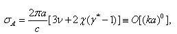 while scattering crossection (deviating from Rayleigh law) was shown[1] to be
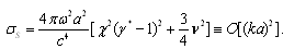 Anyway, in low frequency limit absorption contribution to attenuation usually dominates scattering[1, 18] in medium at rest consisting of small particle, even if heat conduction is ignored. For example, in sound scattering problem stated for fixed or movable sphere[19] in viscous fluid, it was found that neglected viscous term in inhomogeneous (Curl's) equation might lead to erroneous evaluation of few weighty scattered field dipole components. Classical scattering theory proclaims that medium viscosity depresses scattering. It is probably true for fixed or “movable” scatterer, but frequently fails for “moving” scatterer[28]. In[20] the problem of scattering in lossless medium was stated for spatially inhomogeneous sound field in viscous media with tense particles distribution. To develop scattering matrix valid for any value of
  and arbitrary distances between particles right up to their close touch, solution takes into account multiple scattering effects. Requirements of problem analysis strictness are explained there by crucial effect of spherical particle wave scattering on estimates of many physical phenomena and, in particular, low-frequency sound scattering in microinhomogeneous medium, i.e. medium comprising many small particles. In spite of presumable practical importance and expected corrections superiority (at least in losseless media), the number of published papers accounting to scatterers motion with respect to ambient medium is well below the majority of scatterers “movability” papers. First steps in that new direction related to foundations of aerodynamic sound generation[21] were limited to scattered field kinematics (wave convection) description in the vicinity of scatterer and sound source due to medium uniform motion. Various scatterer forms (from compact body to half-plane edge) were analyzed in the presence of multipole sound sources, but additional flow arising due to ambient medium non-uniform motion related to streamlined body or finite size source leading to additional scattering was ignored. One of recent papers[22] devoted to ultrasound biomedical applications also ignores localized flow dynamics related to sphere motion. Effect of sphere motion is reduced there to scattered sound simplified Doppler shift widely covered in literature. In that approach sound field is numerically modeled for multiple spheres motion, leaving main corrections apart. Important contributions were made to the analysis of sound scattering by moving spherical inhomogeneity in relation to mean nonlinear force calculation. For instance, it was shown that direction of mean force on a small sphere does not coincide with direction of radiation pressure force[23]. For small movable sphere effect of viscosity was shown to play significant role for plane traveling incident wave only[24]. Later it was shown[25], that spherical vortex radiation pressure force is zero for plane traveling wave and only non-uniform sound field energy distribution over vortex dimension gives rise to residual radiation force. Our results[26-35] evidence – that restriction of moving scatterers influence on scattered field to kinematics of particle – media relative motions only leads to visible error. Not only moving particle’s surface reflecting sound is involved in effect, but outer non-uniform flow streamlining surface plays noticeable role in scattering as well[26-27, 29]. Additional scattering is even more evident for fixed rigid particles streamlined by flow, say, by uniform flow. It leads to additional attenuation of sound in inhomogeneous media.Microinhomogeneous media discussed therein represents set of scatterers (particles) of various sizes spaced at distances smaller than wavelength. At the same time, thin space between particles considerably exceeds particles average size, providing single scattering approach for low frequency sound waves correctness, at least in the first stage of scattering – at distances where coherent scattered field component still exceeds incoherent. However, we should realize that, if identical inhomogeneities were uniformly distributed in a medium with constant concentration, say, in the form of a periodic lattice, no scattering of that kind would be observed at all, and only a slight change of wave propagation velocity would be observed. In this example, so called “side” spectra of small-scale lattice are reduced to inhomogeneous waves rapidly decaying with distance. According to optical analogy, in such rectilinear crystal, light waves scattered by individual lattice points cancel each other in any direction, except for incident wave direction. In this paper, we are interested in chaotic distribution of particles with their concentration being constant only on the average. Sound wave coherent component decay due to scattering is analyzed below in conditions and distances where field incoherent component is small enough yet, providing multiple scattering contributions being ignored. Exponential decay of field intensity coherent component due to scattering resembles Beer – Lambert extinction law in electrodynamics[11, 18]. Theory of low-frequency sound scattering in such media is based on law that governs individual inhomogeneity scattering. Its size should be small compared to wavelength
  is sound wave number, and
  is the characteristic particles size). For inhomogeneities (particles) at rest, when sound dissipative absorption could be ignored, classical Rayleigh law is valid[1, 4, 7, 8]. According to this law, scattering cross section
  of an inhomogeneity is proportional to body cross-sectional area
  multiplied by dimensionless quantity
  . Usually, microinhomogeneous medium is characterized by concentration of scatterers n and specific scattering crossection
  , determining scattering property of medium unit volume. Due to scattering, wave intensity decreases as distance
  exponential function
 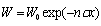 . Logarithmic attenuation index
  characterizing sound wave intensity coherent component decay with distance in terms of decibels per unit length of sound propagation path takes the form
  . For mean radius
  of inhomogeneities and their mean concentration
  , which is expressed through volume of an inhomogeneity and total volume fraction
 occupied by inhomogeneity material in medium as
  , quantity
  is determined by the formula
 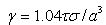 . It was already shown[27-35] that, in general case,
  will depend on parameters of flow near particle and could be expressed in the form of particle section area and dimensionless function
  product:
  , where
  - Mach number,
  - Reynolds number,
  - sound wave angle of incidence with respect to single particle velocity vector. As a result, in simplest case of medium made of identical particles moving with same velocities index
  looks like
  . If there are several (say, N) types of particle of dimensions
  and volume content
  , we shall have expression for cumulative summary attenuation index
  instead of preceding expressions (all sums are taken from
  to
to . Sometimes as in rain case[32, 33] distribution (function) of
  with respect toai is known (
 is also known deterministic function 2 of ai). If particles size distribution is not discrete but continuous function, then instead of sum in expression for
  corresponding integral should be used, so that in deterministic case expression for
  could be easily calculated. In cases of probabilistic particle velocity
  distributions, total
 could be calculated by integration of probabilistic function
  in the limits from
  , say, to infinity. Papers[23-31] were devoted to isolate moving body or localized flow scattering problem solutions giving proper weight to ambient fluid motion. It is obvious that, in general, most of natural microinhomogeneous media elements including “movable” elements examined in[14-22] are in motion. That is why our papers[32, 33] were related directly to low frequency scattering of sound waves in microinhomogeneous moving medium with detailed analysis of rain drops scattering and attenuation. Recent papers[34, 35] are devoted to sound scattering of inhomogeneous media comprising chaotically moving structures (atmospheric turbulence and grouts with Brownian particles). To demonstrate basic scattering law features we shall discuss below simplest case of model media made of identical particles situated chaotically and moving with respect to ambient fluid in orderly or chaotic way with same velocities. To explain law construction methods briefly, mentioning only physically important solution stages and omitting details, we shall use basic results and examples of previous works predictions[23-35]. The purpose of this study is generalization of classical Rayleigh law and Doppler effect as known possible scattered wave non-dissipative reactions to particle motion in ideal fluid to more general case of viscose microinhomogeneous medium comprising inhomogeneities moving orderly or chaotically.
 2. Sound Scattering by Moving Particles in Ideal Fluid
2.1. Orderly Moving Particles
- The flow in major part of space surrounding slowly moving inhomogeneities (say, water drops or chaotically moving particles) is close to potential[2, 3, 6, 27-35]. Therefore, effect of such a flow on scattering is of primary interest. We shall study this phenomenon by considering the flow generated near a spherical particle of radius
 moving with constant velocity V in ideal fluid. Resembling to approach used in[19] for movable particle, we shall describe sound propagation near inhomogeneity by inhomogeneous wave equation frequently called Lighthill’s equation[9], as in[27-31]. For monochromatic wave of frequency
  , this equation has the following form
 | (1) |
 and
and is the acoustic pressure.To complete problem formulation, i.e., to write governing equation with all appropriate boundary conditions, it is necessary to determine relation between acoustic pressure
  and scalar potential
  determining velocity of fluid particles in sound wave:
  . By means of Euler equation accounting for fluid flow in small Mach number
  linear approximation, we deduct that in moving frame of reference
  mentioned relation looks like:
 | (2) |
 and
and  , a mathematical problem can be formulated for potential
  , as well as for the acoustic pressure
  . However in[29, 30], we have applied slightly another more convenient approach. Solution of (1) was formulated for calibration potential
  . This potential is related to sound wave scalar velocity potential
  through relationship
  . Renormalized wave number
  is expressed here through Doppler frequency
 , where
  - unit vectors of incident monochromatic plane wave propagation direction and
  is hydrodynamic Mach number vector. For field component
  , describing sound scattered by velocity inhomogeneities
  characterizing ambient medium flow, in moving frame of references
  equation (1) takes the form
 | (3) |
 is total wave field satisfying Lighthill’s equation, where
  is plane incident monochromatic wave taken in zero-order approximation with respect to hydrodynamic Mach number, and
  is calibration potential corresponding to wave reflected by moving body surface and satisfying homogeneous Helmholtz equation. In the case of potential flow around particle, medium velocity distribution
  is described by the formula
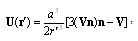 | (4) |
 is unit vector directed from sphere center
  to observation point
  . For convenience, below, as required, the primes indicating spatial coordinates in moving frame of reference are omitted. In
  linear approach, solutions of (3) are represented in the form
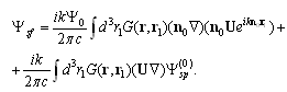 | (5) |
 is amplitude of incident wave and
  is field scattered by sphere surface at rest (reflected wave zero-order approximation in
  ). Integrals in (5) over region outside sphere are calculated by reducing exact function
  to “free space” Green function
 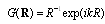 . It is known that, when low-frequency sound is scattered by a stationary particle whose radius is smaller than wavelength of sound, fraction of scattered wave energy is very small, and scattering amplitude is proportional to
  [1, 27]. Then, from comparison of two terms in (5), it follows that for
  second term of solution could be neglected. Discussion of solution (5) possible ambiguity and other details could be found in[27-29]. Options of scattered field separation into individual component follow from the fact - uniqueness of
  and
and  - respective equations solutions require individual conditions at the boundary
  to be defined. However, at perfectly rigid particle surface, only one total field boundary condition is valid
 | (6) |
 is the sum
  in which two terms represent independent unknowns, separation of (6) into two individual conditions for the fields
  and
and  can be done in various different ways. It was shown that solution
  determined in[27, 28] should satisfy as a whole to both initial equations for total field
  and boundary condition (6).
 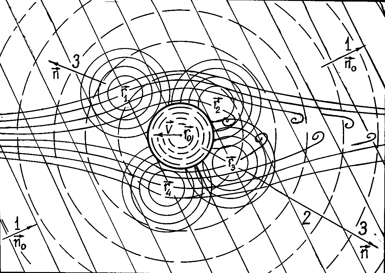 | Figure 1. Scattering principal scheme and scattered field components in the fraction of space around moving particle. Ambient fluid flow is shown schematically behind particle. Direction of particle motion is depicted by velocity vector V. Incident and passed over wave directions are shown by unit vector  while field observation directions - by unit vectors while field observation directions - by unit vectors  . Few flow local scattering centers situated near sphere (to be integrated over area to obtain total scattering amplitude . Few flow local scattering centers situated near sphere (to be integrated over area to obtain total scattering amplitude  ) are shown by radius vectors ) are shown by radius vectors  , while particle surface scattering center is shown by radius vector , while particle surface scattering center is shown by radius vector  . In addition to incident and passing waves potential . In addition to incident and passing waves potential  - 1, there are two scattered field potential components - 1, there are two scattered field potential components  - 2 and - 2 and  - 3 expressed in paper through scattering amplitudes - 3 expressed in paper through scattering amplitudes  related to body surface and adjacent flow scattering respectively related to body surface and adjacent flow scattering respectively |
 scattered by flow inhomogeneities in a lot of cases (e.g., when
  ). From expression
  , which is valid for
  , we determine scattering amplitude
  for incident plane wave
  , scattered by flow inhomogeneities (4) surrounding moving sphere. Scattering amplitude acquires following form
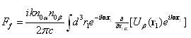 | (7) |
 occupied by flow.From expression (4) and estimate of integral (7), it follows that region adjacent to sphere surface makes a key contribution to (7). Therefore, extension of integration region in (7) to entire space, including region
  (as it is done sometimes) may lead to error. We have performed integration in (7) and determined scattering amplitude
  for arbitrary values of
  [30]. Taking integral by parts we represent it in the form
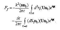 | (8) |
 positioned infinitely far from body vanishes, because fluid velocity
  decreases with distance from sphere center as
  according to (4) while area of the surface
  increases as
  . Wave vector
  has the sense of "momentum" transferred to medium. Its magnitude is
  and
and  is scattering angle determined by equation
  . Substituting potential flow velocity (4) in (8), we obtain a specific expression for scattering amplitude
  . Calculation of integrals is discussed in[30]. Using results of volume and surface integration in (8) we obtain
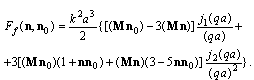 | (9) |
 and
and  are first- and second-order spherical Bessel functions. Using (9), it is possible to determine partial scattering amplitude that characterizes low-frequency sound scattering by fluid flow generated near small inhomogeneity. Assuming that
  , we expand Bessel spherical functions involved in (9) in power series with respect to this small parameter and obtain following formula for scattering amplitude
 | (10) |
 for sound scattered by moving inhomogeneity surface was performed in[29] for arbitrary values of
  . In approximation
  , exact expression takes the form accurate up to
  terms
terms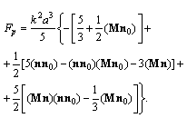 | (11) |
 .From (10) and (11), it follows that corrections to scattering amplitude due to motion of scatterer taking into account potential flow generated around it are proportional to
  . They are anisotropic, because expansion in spherical harmonics series contains monopole, dipole, and quadrupole components. Taking squared magnitude of amplitude (10) and integrating it over solid angle, we determine partial scattering cross section
  for sound scattered exceptionally by potential flow (4). Calculations 27 show that
  is expressed as
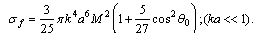 | (12) |
 is an angle between vector
  and body velocity V (
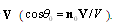 ).It also follows from (10) and (12) that partial scattering crossection characterizing sound scattered by potential flow near moving microinhomogeneities is proportional to the square of Mach number. However, as it was mentioned above, sound is scattered not only by medium flow generated by particle motion, but also by moving surface of particle itself. When sound is scattered by fixed rigid microinhomogeneity of small radius (
 ), scattering amplitude is proportional to
  , so that scattering crossection is proportional to
  in compliance with classical Rayleigh law[1]. For an inhomogeneity with finite density and compressibility, under condition
  , scattering cross section
  has the form 1
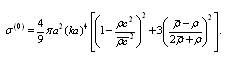 | (13) |
 and
and  are sound velocities in fluid and in particle material, respectively;
  and
and  are their densities; and
  is wave number. Motion of particle with a velocity
  gives rise to corrections to amplitude
  and scattering crossection
  , due to sound scattered by both flow and moving particle surface. Thus, calculation of total scattering cross section for sound scattered by moving inhomogeneity with allowance for both wave diffraction by its moving surface and wave scattering by inhomogeneities of surrounding fluid related to accompanying flow leads to the appearance of additional terms in expressions for scattering amplitudes of the type of (10) and (11). In addition to term
  , which is described for instance by (13), and is zero-order in Mach number, and to the terms that are quadratic in Mach number - arising due to amplitude
  linear corrections squared in expression for
  , cross terms proportional to Mach number will arise as well. Total scattering crossection for a small particle moving with the velocity
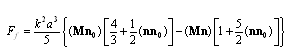
  , surrounded by potential flow (4), acquire fairly simple form [27]
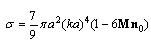 | (14) |
 . For sphere with arbitrary density and compressibility generalized law takes the form
 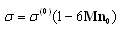 , where
  is given by (13), while
  is slightly modified.It is useful to calculate crossection
  for “transparent” inhomogeneity. It resembles (12) and is related to particle of density and compressibility just the same as ambient fluid (
 ) for which
  given by (13) will turn to zero. It equals to 27
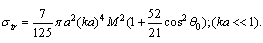 | (15) |
 or linear in
  . However, (15), just like (12), could be used as correction estimate for (14), being fair up to
  order only – if it is necessary to write it out with accuracy up to
  . It is necessary for instance in scattered sound field calculation for wave propagating in normal direction to particles velocity, say, for horizontal sound waves in rain. It follows from (15) that in such approximation scattering will increase with velocity irrespectively of particle velocity and wave propagation relative directions.
 2.2. Chaotically Moving Particles
- As we have noted above, in the Introduction logarithmic attenuation rate
 for inhomogeneous media with identical orderly moving particles (say, uniform flow or rain) could be calculated on the basis of particles scattering crossection
  . In order to generalize this expression to the case of inhomogeneous media with particles chaotic motion it is necessary to average expression for
  with respect to various sound wave incidence angles
  supposing that all scattering acts and all directions of particle motion are equiprobable. It is equivalent to
  averaging over spherical solid angle (
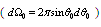 ) to obtain averaged value of scattering crossection
  independent of
  according to expression
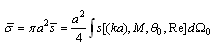 | (16) |
 , we obtain average crossection value for chaotically moving particles
  coinciding in accuracy up to
  with classical Rayleigh law[1, 4]
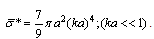 | (17) |
 , (17) will hold independent of
  value and its relationship to
  . To evaluate
 with accuracy up to
  it is necessary to supplement (14) by expressions (12) or (15). Physically first option takes into account definite portion of scattered field reflected by particle surface and rescattered by flow, while second – neglects reflections from particle - for particle is completely transparent in acoustic sense. Averaging results are comparable and executing necessary integration of (12) and (15) taking into account that
  , we derive average crossection
  and
and  for chaotic particle motion valid with accuracy up to
  respectively
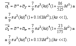 | (18) |
 , where factors
  correspond to
  and
and  averaged values. For particles with arbitrary compressibility and density generalized Rayleigh law for
  , written with accuracy up to
  , takes the form
  , where
  is given by (13), while factors
  , corresponding to averaged
  and
and  values, slightly tell from factors in (18), being: β1 ≈ 0.29, β2 ≈ 0.23. Taking into account the form of
  expressed through
  , we can obtain
  , say, for rigid particle (18) in the following form:
  . In ideal fluid dependence of
  on Reynolds number is missing. Due to linearity of basic equation (1), in the case of particles weak chaotic motion, superposition of more rapid ordered motion (say, for particles buffeted by local wind or flow) over their, modified Rayleigh law (14) with Mach number of that rapid motion, will be valid as well. Evaluation of raindrops motion effect on sound scattering in ideal fluid is provided in[32].
2.3. Scattering Frequency Dependence
- Let us consider now frequency dependence of sound scattered by inhomogeneities of fluid accompanying flow. It is similar to frequency dependence of sound scattered by moving body itself, because it is determined by same time factors multiplying scattering amplitudes
 and
and  . If, in these factors
  , we expand quantity
  in small parameter
  , we can find that time dependence is determined by ordinary exponential time factor
  . Scattered field frequency depends on both angle of wave incidence and angle of wave observation and has the form of
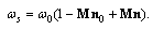 | (19) |
 . From (19) it follows that, at stationary position
  , frequency of scattered sound
  varies as a function of observation angle and may coincide with incident wave frequency
  in two cases. Firstly, this may occur when sound is scattered at zero angles, i.e., when
  . Secondly, the frequencies may coincide when sound is scattered at an arbitrary angle under the condition that velocity vector V is perpendicular to the difference between the unit vectors n and
  . In particular, if scattering region is observed in transmission geometry, frequency shift
  will be absent at the instant when body crosses transmitter - receiver line irrespective of crossing angle. Comparison of (19) to (10), (11) and their sum leading to (14) provides important conclusion. Scattered field reacts on value and direction of scatterer motion velocity not only through purely cinematic condition (19) – classical Doppler effect, but through scattering amplitude (10), (11) and crossection (14) respectively, that are related to energy space distribution and are dynamical in nature. Scattered wave is shown to acquire phase – amplitude dependent (anisotropic) form with respect to observation direction instead of purely phase dependent form (Doppler effect) expected for small moving particle in classical moving particle scattering, ignoring ambient flow. This argument generalizes scattered field properties for moving scatterer even in ideal milieu.
 3. Sound Scattering by Moving Particles in Viscose Fluid ( )
)
3.1. Theory
- To calculate sound scattering in viscous fluid flow caused by small particle, we assume, as above, that velocity of moving inhomogeneity
 is constant and small compared to medium sound velocity
  . If radius of microinhomogeneity is sufficiently small, Reynolds number
  is also small, and we have Stokes flow around particle while velocity distribution
  in coordinate system
  in the fluid acquires the following form[1, 5]
 | (20) |
 is unit vector directed to observation point. In laboratory frame of reference, velocity
  is expressed as
  - primes are omitted below.Basic Lighthill’s equation (1) is correct up to linear terms in hydrodynamic Mach number, but it initially ignores viscosity and variation in entropy of fluid due to dissipation processes related to heat conduction and medium viscosity. Accounting for dissipative processes in Mach number zero-order approximation leads to additional attenuation of propagating waves. For plane monochromatic wave
 , inclusion of these terms in (1) leads to wave number
  correction, i.e., to introduction of non-zero imaginary part[7],[9]
 where
where  and
and  are viscosity factors,
  is thermal diffusivity, and
  is specific heats ratio. It leads to renormalization of wave number
  in (1), which is assumed to be done in subsequent calculations. Equation that is more general than (1) is known as Blokhintsev – Howking’s equation[7],[9]. It also contains cross terms that are linear in Mach number
  and proportional to the first power of dissipation factors. If these factors and Mach number are small, then aforementioned additional terms remain small compared to terms that are already presented in (1) and, hence, can be safely ignored in Mach number linear approximation. Thus, sound propagation in viscous medium considering adjacent flow near a moving body can also be described by (1) even if flow vorticity near body is nonzero, e.g. (20), where velocity is a sum of two terms
  , in which
  is second term of (20) and
  is third term of (20). First term of (20), i.e.
  , related to shift of coordinate system is unimportant for scattering evaluation.Expression for velocity component
  is similar in structure to (4) and differs only in the coefficient, which is (-1/2), so that
  is 2 times smaller than potential flow velocity. Therefore, representing total sound scattering amplitude
  by the sum of two terms,
  which is determined by the respective components
  , we easily obtain expression for amplitude component
  determined by the flow
  . Using result of 27, where the scattering amplitude was found for sound scattered by potential flow inhomogeneities (4), and taking into account the aforementioned factor (-1/2), we see that amplitude component
  makes one half of (11). The scattering amplitude component
  is calculated on the basis of (7), in which velocity
  is taken in the form
  . This velocity component decreases slower with distance from the particle(
 ). Such behavior leads to increase of integral value being determined by vortex character of viscous flow. Indeed, direct calculation shows that
  and flow vorticity
  due to velocity component
  is given by expression
  . After integration (c.f. details[28, 32]), we obtain that
  generated by flow component U2 is given by
 | (21) |
 associated with vortex flow scattering is greater than
  by a factor of
  and does not depend on frequency. Hence, as frequency decreases, the ratio of these amplitudes rapidly increases. Since total scattering amplitude
  is determined by the component
  , while
  makes half of scattering amplitude associated with scattering of sound by potential flow only, we can conclude that, for
  , inclusion of fluid viscosity leads to considerable increase in sound scattering amplitude.However, accurate calculation of previously rejected part of integral (5), i.e., the part related to the velocity
  rather than to its derivative (8), shows that, in fact, this part is not small and should also be taken into account as well. Direct calculation of integral (5) with allowance for second term in its integrand formally leads to integral divergence as consequence of slow velocity (20) decrease with distance. It should be reminded that Stokes-type velocity distribution in a viscous fluid (20) holds only in the particle surface adjacent region, whereas, away from the body, velocity decreases faster than
  [1-5]. Hence, region of integration in (5) can be physically restricted to a distance of an order of
  , within which distribution (20) is actually valid. As a result, scattering amplitude
  becomes finite. The estimate of integral (5), as calculated value of expression (21) for the amplitude
  , proves to be much greater than scattering amplitude of sound wave scattered by potential flow inhomogeneities. Corresponding partial scattering cross section considerably exceeds value of (12) and, for
  , is expressed as
 | (22) |
 as well, mentioned in the Introduction and for not too small
 exceeds even absorption crossection mentioned there. In calculation of total scattering cross section, it is necessary to consider three cases depending on relative values of
  and
and  [28]. Taking into account that
  , where
  is given by (10) and the sum
 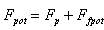 is given by the sum of (10) and (11), we denote
  and obtain total scattering amplitude in the form
 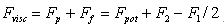 . Squared magnitude
  used in scattering crossection calculation is
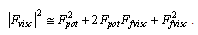 | (23) |
 , which, in their turn, are proportional to the product of cross-sectional area of the inhomogeneity by
  respectively in comparison to terms retained in (23) and proportional to
  respectively.
3.2. Orderly and Chaotically Moving Particles
- If
 , we have
  , and, in scattering crossection calculation
  , it is possible to ignore not only the term proportional to
  , but also the first term of (22), which is proportional to
  . Thus, we retain only the second and last terms of (23), which are proportional to
  and
and  respectively. Scattering crossection takes the form of
 | (24) |
 and
and  - angle averaged expression for
  in the case of particles chaotic motion will take the form
 | (25) |
 related to independent of particle body scattering viscous flow (22) contribution. It means that, in this case, moving particle bodies are unimportant for scattering evaluation.If
  , we obtain
  . In this case, it is possible to retain only first term of (23), which is proportional to
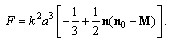
  . The scattering obeys modified Rayleigh law for the case of potential flow around the body, and the expression for scattering crossection coincides with (14)
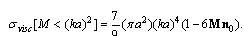 | (26) |
 , it is easy to see that for particles chaotic motion angle averaged (26) coincides with (17) - classical Rayleigh law[1].Finally, if
  , we have
  . Then, in (24), only terms proportional to
  can be ignored in favor of three terms proportional to
  and
and  to be retained. In first term, it is possible to ignore summand proportional to
  in parentheses of (14). Expression for scattering crossection takes the form of
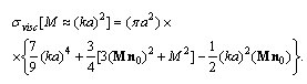 | (27) |
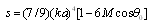
 for chaotic particles motion acquires the form of
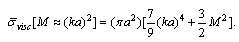 | (28) |
 proposed above, and expressed for chaotic inhomogeneities motion through function
  , we shall see that in viscous flow at
  we have: for
  by relationship (25) as
 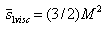 ; for
; for  - as
- as 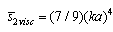 and for
  by relation (23) as
 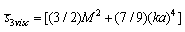 . Explicit dependence of
  on Reynolds number at
  is missing. While (24), (26) and (27) reflect scattering laws for inhomogeneities orderly motion, relationship (25) , (17), (28) reflect - laws for chaotic motion in viscous fluid. Evaluation of raindrops motion effect on sound scattering in this range of Reynolds number is provided in[32].
4. Sound Scattering by Moving Particles in Viscose Fluid ( )
)
4.1. Theory
- In[32] we have noted that, for raindrops with diameters of 1 - 5 mm and with dip velocities of an order of several meters per second[2], the estimates of attenuation values executed for
 are hardly valid. The actual influence of the viscous flow on sound scattering by rain drops of this size cannot be estimated by Stokes law, because drag coefficient for falling rain drops, which determines surrounding fluid flow, proves to be many times lower[2]. The above estimates of viscosity effect on scattering are restricted by limiting diameter of rain drops, up to 0.1 mm (0.01-0.1 mm), and limiting velocity of drops motion, up to 0.3 m/s (
 ). On further increase in drops velocity or in size, with Reynolds number increase, flow acquires laminar wake features[2, 31, 33].Corresponding calculations could be performed in the same manner as in the cases of inhomogeneous ideal or viscous (
 ) fluids on the basis of Lighthill’s equations (1) and (3) with solutions (5), (8). But now velocity distributions (4) and (20) respectively are to be substituted by new expressions for the case of laminar wake (
 ). As before, we suppose that small axisymmetric (say, spherical) particle of transverse dimension
  is moving in viscous fluid with uniform velocity
 Flow structure was discussed in details in[1, 2, 31]. In this approach, velocity distribution
  far from the particle inside the wake is[1, 2]
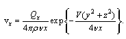 | (29) |
 - fluid density,
  - drag force in
  direction applied to fluid by particle,
  - transverse section area of particle with respect to motion direction,
  –form dependent particle drag factor. In general
  depends on Reynolds number as well[2, 31].Velocity distribution outside the wake could be regarded as potential. Restricting flow distribution outside particle by most slow decreasing components of monopole and dipole nature we can write down general expansion for axisymmetric particle flow distribution[1]
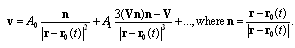 | (30) |
 and
and  are to be found as usual by means of boundary conditions. For instance, first factor
  is found using the condition that total flows over the surface of large sphere as over any closed surface containing moving body is zero. Simple calculations based on (29) and (30) will express it in the form
  [1, 2]. Far from axisymmetric body in viscous medium potential part of flow distribution acquire monopole structure and looks like
 | (31) |
 to be described approximately by (29) and (30). According to (8), we see that additional volume integrals related to (30) outside wake and (29) inside wake, together with surface integrals, related not only to body surface but to wake surface as well, are to be considered[31]. Calculations[31,33], evidence that scattering law version substituting law (14) for particles moving in viscous fluid at large
  choice will depend on
  relationship[31,33].
4.2. Orderly and Chaotically Moving Particles
- For
 there are two physical objects responsible for scattering: body of particle and it’s laminar wake. To prevent divergence in wake scattering evaluation we have used physical restriction of integration volume by introduction of finite wake length
  [31]. This assumption provides zero angle integral scattering amplitude finite value. Scattering amplitude turns out to be finite even in the case of “look through” geometry (
 ). It was shown that scattering crossection exceeds
  times (
 ) crossection (14), based on potential flow around particle in ideal fluid[33]. Thus, for
  and
and  , instead of (14) we shall obtain expression for sound wave scattering crossection
  by particle moving in viscous fluid at
  and generating laminar wake
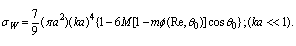 | (32) |
 - the factor of an order of unity is depending in general on wave incidence angle
  and Reynolds number of flow. Particularly, in (14), expressing modified Rayleigh law for particles moving in ideal fluid[33], the value of
  is zero. Relationship (32), in its turn, expresses generalized scattering law for inhomogeneous medium with slowly moving particles (
 ) at large Reynolds numbers for
  and
and  .Consequently, for chaotic particle motion, taking into account that
  , expression of
  averaged over incidence angles acquires the form
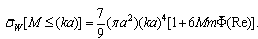 | (33) |
 angle averaged function
  - with value of an order of unity depending on flow Reynolds number
  only. Expression (33) depends on frequency in a manner close to modified Rayleigh law (14), but is distinguished by important correction
  in square parenthesis depending on
  .For
.For  , the flow outside wake, determined by first (monopole) term of (30), is responsible for scattering. Its contribution to the crossection comprises three terms[31, 33], exceeding contributions of particle body and its wake. Omitting their calculation, we write down the result[33]
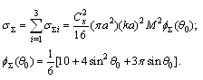 | (34) |
 , is essentially positive in angle
  range from 0 to
  . Its value changes from 5/3 at
  to
to 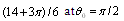 and, once more, to 5/3 at
 . At
. At  value of
  equals to
  . It is worth to note that scattering crossection
  acquires maximum for sound wave transverse (normal) direction to particles velocity incidence (
 )[33].Thus, for
  , relationship (34) expresses generalized scattering law for inhomogeneities (particles), slowly (
 ) moving in viscous medium at large Reynolds numbers. Taking into account that
  , and
, and  , angle averaged expression of
  for particles chaotic motion acquires the form
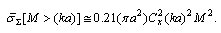 | (35) |
 through
  [2]. As a whole, taking into account form of averaged scattering crossection
  expressed by function
  at
at  , we could write down, say, for
  , by virtue of (33)
 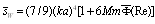 ; while for
  in accordance to (35) – as
  . At
. At  , explicit dependence of s on
  in viscous media is presented in the form
  in (33) and in the form of
  in (35). Relationship (33) and (35) reflect forms of generalized scattering law for chaotically moving particles in viscous fluid at
  . Scattering law forms derived here are distinguished by much stronger inequality,
  to be executed at
  , than inequality
  at Stokes flow conditions
  . Evaluation of raindrops motion effect on sound scattering in this range of Reynolds number is provided in[33].
5. Application examples
- Scattering laws derived above are supported by examples of their practical application.
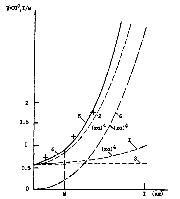 | Figure 2. Typical sound attenuation index  (multiplied by 103) frequency (wave number parameter (multiplied by 103) frequency (wave number parameter  ) dependencies developed in the frames of atmospheric turbulence scattering corpuscular models for strong (curves 2, 4, 5) and weak (curve 1) turbulence regimes[34] ) dependencies developed in the frames of atmospheric turbulence scattering corpuscular models for strong (curves 2, 4, 5) and weak (curve 1) turbulence regimes[34] |
 frequency dependencies developed in the frames of atmospheric turbulence scattering corpuscular models[34]. Dotted curves 1 and 2 show dependencies derived in accordance to corpuscular models
  and
and  in ideal fluid approach for weak (modeled by chaotically moving transparent spheres of various dimensions) and strong (modeled by chaotically moving Hill vortices of various dimensions) turbulence regimes respectively. Factors
  and
and  of curves 1 (weak turbulence) and 2 (strong turbulence), are distinguished sharply – at least in two orders. Horizontal dotted line 3 shows the value of scattering spectrum pedestal, related to sound scattering by smallest internal (Kolmogorov’s scale) vortices (25). Solid curve 4 shows attenuation index
  dependence
 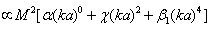 , accounting to specific type of correction to curve 2 related to atmosphere viscosity. Such corpuscular model is fair for parameter
  range lower than Mach number
  of turbulence external scale (33). Solid line 5 shows attenuation index dependence
 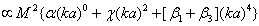 , accounting to other type of correction to curve 2 related to atmosphere viscosity. Such corpuscular model is fair for parameter
  range exceeding Mach number
  of turbulence external scale (35). Curve 6 shows typical attenuation index
  frequency dependence derived from known wave models for turbulence sound scattering
  . Widely known discrete experimental data of Zieg and Blokhintsev[7] for low frequency sound attenuation in atmosphere explained by corpuscular scattering models – curves 4 and 5 are shown by crosses. It is seen also that Zieg data poorly correlate with “wave scattering” models – curve 6.
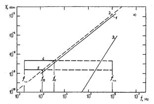 | Figure 3. Frequency dependence of sound attenuation index  in frequency range 102 – 3 107 Hz for water solution of identical suspended particles with radius in frequency range 102 – 3 107 Hz for water solution of identical suspended particles with radius  at standard room temperature most probable Brownian motion velocity at standard room temperature most probable Brownian motion velocity  Both examples evidence importance of scatterers motion in evaluation of sound scattering or sound wave attenuation with distance Both examples evidence importance of scatterers motion in evaluation of sound scattering or sound wave attenuation with distance |
 in frequency range 102 – 3 107 Hz for water solution of identical suspended particles with radius
  participating in Brownian motion is shown on Figure.3[35]. Horizontal axis shows frequency values (Hz) logarithmic scale. Vertical axis shows attenuation index values in the range from 10-10 to 10-2 dB/m linear scales. Curves 1, 2 show frequency dependence of absorption index theoretical and experimental values in water, related to irreversible sound energy losses due to heat conduction and viscosity, respectively. Curve 3 shows frequency dependence of index
  , related to sound scattering attenuation evaluated by classical Rayleigh law for immobile suspension particles[1]. Dotted lines 4 and 5 show frequency dependencies of additional attenuation related to particles Brownian motion with definite initial velocities. It was chosen from Maxwell distribution as most probable velocity value for outer standard room temperature
  = 0.005 m/s for particles relative volume abundance
  and
and  respectively. Solid parts of dotted lines show curves frequency region where effect of additional scattering is most observable with respect to solvent (water) sound absorption. They are restricted by frequency values from lower boundaries
  and
and  respectively for corresponding particle volume content
  and
and  . Upper frequency boundary value
  is the same for each curve.
 6. Conclusions
- Thus, in general, motion of inhomogeneous media with respect to direction of wave propagation leads not only to Doppler frequency shift of scattered wave, but modifies Rayleigh law in any of their intersection angles range, even if particles size exceeds viscose wave length. Probably, microinhomogeneities scattering ability calculated above could be slightly overestimated, since it ignores irreversible (dissipative, say, viscous) losses of particles mechanical energy in sound wave generated by wave oscillations, which are expected simultaneously with secondary sound radiation. As we have noted, these losses lead to slight decrease in amplitude and, hence, to decrease in scattering[1-9]. However, they could be safely neglected together with effect of scatterers’ “movability” mentioned in the Introduction.On the other hand, presence of medium viscosity affects structure of flow near moving inhomogeneity. In particular, potential flow is transformed to develop vorticity and, in addition, the decay of flow parameters with distance becomes slower. It leads to linear in Mach number non-dissipative change in scattering cross section[28, 32-33] and to change of scattered field intensity frequency dependence from
 in[1-9], to
  (22), (25) in[28, 32] and to
  (34), (35) in[33]. Evidently, second effect of fluid viscosity is much more distinct than the first (“movability” effect), especially for ordinary (non-resonant) inhomogeneities, such as various rigid particles (e.g. Brown’s particles[35]), sand particles blown by the wind or falling drops of rain[32-33]. As it was shown, corrections to scattering cross section are expected even for potential flow around moving inhomogeneity. Being proportional to particles hydrodynamic Mach number, they generalize modified low frequency sound attenuation Rayleigh laws in ideal microinhomogeneous medium (14) and Doppler effect (19). Sometimes, in viscous microinhomogeneous medium, low frequency sound attenuation could be almost frequency independent and defined mostly by flow adjacent to moving particles, while particles body scattering contribution could be neglected[28, 32-35]. Viscous flow near inhomogeneities not only intensifies sound absorption owing to additional losses as was known before, but considerably enhances non-dissipative scattered field as well[32-35]. These conclusions extend classical views determining effect of particles motion and viscosity on scattering intensity in microinhomogeneous medium, which are widely used for stationary inhomogeneities. Classical scattering theory[1] basic assumption proclaiming that “…scattering related to body motion comprises only small correction to scattering related to influence of the body itself. This correction will be further ignored. That is, we shall suppose scattering body to be immobile” is hardly true for moving media sound scattering. It is based on analogy between scattering processes in acoustics and electromagnetic theory[4, 8, 10, 12, 13] widely used in scattering and attenuation prediction, meaning that mentioned corrections to scattering amplitude are of an order of Mach number. However, while in electromagnetic theory Mach number correction could be safely ignored, in realistic media acoustics, as it is shown above, it should be taken into account and mentioned analogy fails. Slighting of this important sound field property in practice may lead to scattering evaluation errors even for subsonic inhomogeneity motion. Ambient flows near moving scattering particle frequently[28, 32-33] turn out to be key factor in low frequency sound scattering, while in classical scattering theory[1, 4] they are not even mentioned. Instead of classical Rayleigh law for fixed particles with structure defined by particles dimensions and inner properties only, moving media low frequency sound scattering law versions derived above are defined by particles motion Reynolds number
  value, wave incidence angle
  and Mach number
  – incident wave parameter
  relationship[32-35]. For realistic media (usually moving) with particle dimensions and velocities actual diversity, where resulting attenuation will be combined of effects discussed above in accordance to procedure mentioned in the Introduction, we can conceive a conclusion. Attenuation parameter frequency dependence
  to be observed in microinhomogeneous moving media experiments in low frequency range could look more complex than simple fourth power monomial
  , predicted on the basis of fixed particles scattering law. In general, it could look as biquadrate trinomial
  , even if sound absorption could be neglected and inhomogeneities characteristic dimensions exceed viscose wavelength
  of the media.