-
Paper Information
- Next Paper
- Paper Submission
-
Journal Information
- About This Journal
- Editorial Board
- Current Issue
- Archive
- Author Guidelines
- Contact Us
American Journal of Fluid Dynamics
2012; 2(3): 7-16
doi: 10.5923/j.ajfd.20120203.01
Gas-non-Newtonian Liquid Flow Through Horizontal Pipe – Gas Holdup and Pressure Drop Prediction using Multilayer Perceptron
 Abstract
 Reference
 Full-Text PDF
 Full-Text HTML
Nirjhar Bar, Sudip Kumar Das
Department of Chemical Engineering, University of Calcutta, Kolkata, 700009, India
Correspondence to: Sudip Kumar Das, Department of Chemical Engineering, University of Calcutta, Kolkata, 700009, India.
| Email: |  |
Copyright © 2012 Scientific & Academic Publishing. All Rights Reserved.
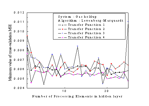
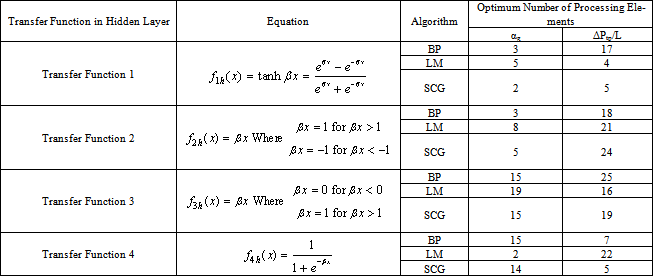
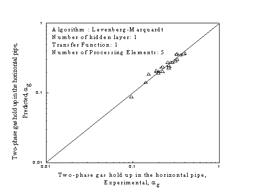
Prediction of the gas holdup and pressure drop in a horizontal pipe for gas-non-Newtonian liquid flow using Artificial Neural Networks (ANN) methodology have been reported in this paper from the data acquired from our earlier experiment. The ANN prediction is done using Multilayer Perceptrons (MLP) trained with three different algorithms, namely: Backpropagation (BP), Scaled Conjugate gradient (SCG) and Levenberg-Marquardt (LM). Four different transfer functions were used in a single hidden layer for all algorithms. The Chi-square test confirms that the best network for prediction of gas holdup is when it is trained with Levenberg-Marquardt (LM) algorithm in the hidden and output layer with the transfer function 1 in hidden layer having 5 processing elements. The Chi-square test also confirms that the best network for prediction of pressure drop is when it is trained with Backpropagation (BP) algorithm in the hidden and output layer with the transfer function 4 in hidden layer having 15 processing elements.
Keywords: Gas Holdup, Pressure Drop, Gas-Non-Newtonian Liquid Flow, Backpropagation, Scaled Conjugate Gradient, Levenberg-marquardt
Article Outline
1. Introduction
- The co-current gas-liquid flow through pipeline has many different industrial applications, like chemical, petrochemicals and nuclear plants, crude oil pipelines etc. The gas-liquid flow become very complex in nature and the three important hydrodynamic parameters are the void fraction, pressure drop and flow regime. These parameters have been studied extensively by experimentally and theoretically. In order to accurately estimate the pressure drop and void fraction, it is necessary to know the flow pattern accurately[1]. Enormous literatures available in this field have been summarized in several books[2-5]. Most of these studies are with gas-Newtonian two-phase flow. However, very little information is available when the liquid is non-Newtonian in nature. The experimental studies on the hydrodynamic parameters estimation for gas-non-Newtonian liquid flow though horizontal pipeline are reported by only few researchers[6-33]. All these studies show that the gas-non-Newtonian liquid two-phase flow hydrodynamics in pipes behave differently from the hydrodynamics of a gas-Newtonian liquid flow. Ward and Dallavalle[6] observed drag reduction by injecting air into clay suspensions flowing in laminar regime. Oliver and Young Hoon[7] reported the several differences between the flow patterns that occur in gas-Newtonian and gas-non-Newtonian liquid flow. According to their experimental findings Newtonian liquids tend to produce circulating patterns whereas the non-Newtonian liquids produce stream line deflections around the gas slug. They tried to correlate their experimental data by Lockhard-Martinelli correlation[8]. Rosehart et al.[9] also observed similar deviation. Mahalingam and Valle[10] reported that the flow patterns for-gas-Newtonian liquid flow were similar to that of gas-Newtonian liquid system. They observed that the two-phase pressure drop were greater than those of the gas-Newtonian liquid flow. They also observed a sharp increase in pressure drop in the bubble flow region but as the flow pattern changed to slug and wavy flow region, increase in air velocity resulted in sharp decrease in pressure drop, the gas holdup increased with increasing gas flow rate and decreasing pseudo plasticity. Rosehart et al.[11] studied two-phase gas -non- Newtonian liquid slug flow using drag reducing polymer solution, i.e., liquid phase containing small amount of polyacetamide, a long chain polymer. They reported that the drag reduction in two-phase flow greater than in single phase flow and also showed the importance of the acceleration term in the axial pressure gradient.Srivastava and Narsimhamurthy[12,13] reported their experimental studies on the two-phase gas-non-Newtonian liquids in horizontal pipes with turbulence promoters and analysed their pressure drop and holdup data using modified Lockhart-Martinelli[8] correlation. Tyagi and Srivastava[14] analyzed the pressure drop data for annular flow of gas-non-Newtonian liquid and proposed an analytical model relating the film thickness with flow rates, physical properties of the fluids and the energy losses. Otten and Fayed[15,16] reported studies on both the pressure drop and drag reduction and later on the slug velocity and frequency in concurrent flow of air-carbopol 941 solution. Heywood and Richardson[17] studied the flow of air-kaoline solutions and observed a large reduction in pressure drop by injecting the air into the slurry. Similar drag reduction was observed by Farooqi et al.[18] for air-anthracite slurry flow. Eisenberg and Weinberger[19] developed an expression for the prediction of pressure drop and holdup for annular two-phase flow of gas-non-Newtonian liquid. They modified the Lockhart-Martinelli correlation to take into account the shear rate dependence on the apparent viscosity of the liquid phase. Heywood and Charles[20] published a gas-non-Newtonian liquid stratified flow model to predict the liquid holdup and pressure drop. Farooqi and Richardson[21,22] reported their experimental studies on gas-Newtonian and gas- non-Newtonian liquid flow and analysed their data by modifying the Lockhart-Martinelli correlation. Chhabra et al.[23] studied the co-current flow of air and shear thinning china clay suspensions in water in a large diameter horizontal pipe. They observed that the Faaooqi and Richardson[22] correlation agrees well with the experimental two-phase data. Chhabra et al.[24] studied the pressure drop and hold up in isothermal two-phase flow of air and aqueous polymer solution in horizontal pipe. Their experimental results agreed well the equations suggested by Farooqi and Richardson[22]. Das et al.[25,26] studied gas-non-Newtonian liquid flow through horizontal tube and developed empirical correlation for the prediction of two-phase pressure drop and holdup. Dziubinski[27] studied experimentally and presented an expression of drag ratio for two-phase pressure drop of intermittent gas-non-Newtonian liquid flow based on the loss coefficient concept. Jinming and Jingxuan[28] experimentally studied the two-phase gas-non-Newtonian liquid such as sewage sludge and black water in sewers in pipes and modified the Lockhart-Martinelli parameter for the prediction of two-phase pressure drop. Ruiz-Viera et al.[29] studied lubricating grease-air flow through different geometries of smooth and rough surfaces and observed drag reduction. Xu et al.[30] studied gas-non-Newtonian liquid flow through horizontal tube of 50 mm diameter. Xu et al.[31] studied co-current air-non-Newtonian liquid flow in inclined tubes of different diameters. Xu et al.[32] observed the drag reduction by gas injection to non-Newtonian liquid in stratified and slug flow regimes. They also proposed models for each flow regimes to predict the two-phase pressure drop and drag reduction. Jia et al.[33] reported the three dimensional computational multiphase fluid dynamics CMFD simulations to estimate the two-phase pressure drop in slug gas-non-Newtonian liquid flow system. ANN models have been extensively studied in different fields of engineering, finance etc. in last two decades with an objective of achieving human like performance. ANNs are derived from the biological counterparts, and based on the concept that a highly interconnected system of simple processing elements, known as nodes or neurons, which are able to learn highly complex nonlinear interrelationships existing between input and output variables of the data set[34].Cai et al.[35] used neural network to identify flow regimes in air-water flow. Leib et al.[36] used ANN model along with the mixed-cell model to predict the slurry bubble column performance for Fischer-Tropsch synthesis. Various ANN modelling were used to predict various hydrodynamic parameters in packed bed and fluidized bed reactors[37-40]. Shippen and Scott[41] used ANN as predictive tool to predict liquid holdup in two-phase flow. Osman and Aggour[42] developed ANN model to predict the pressure drop for gas-liquid flow through horizontal and near horizontal pipes from a data bank consisting of 450 sets of oil field data. They observed that the ANN model predict the pressure drop very accurately than the existing available correlations and mechanistic models. Malayeri et al.[43] used radial basis function neural network to predict the cross-sectional and time-averaged void fraction at different temperature in air-water two-phase flow. Alizadehdakhel et al.[44] studied gas-liquid flow through 2 cm diameter tube and they modelled using CFD and ANN techniques. They concluded that the prediction of two-phase pressure drop using CFD is more accurate than the ANN prediction and moreover it gives the insight of two-phase flow. Shaikh and Al-Dahhan[45] observed that the ANN prediction of the gas holdup in bubble column reactors give better predictability than the correlations available in the literature. Nasseh et al.[46] used neural network optimized by genetic algorithm to predict the pressure drop in venturi scrubbers.The pressure drop for non-Newtonian liquid and gas-liquid flow through different piping components like elbow, orifice, gate valve and globe valve was successfully predicted by Bar et al.[47,48] using the same Multilayer Perceptron. The neural network used by them had four different transfer functions in a single hidden layer. Only backpropagation algorithm was used for training. Bar et al.[49] also used the same method algorithm to predict the frictional pressure drop for non-Newtonian gas-liquid flow through 45° bend in the horizontal plane.ANN models can able to learn from examples, incorporate large number of variables, and provide an adequate and quick response to the new information. The advantages of neural networks are (1) the ability to represent both linear and nonlinear relationships, (2) the ability to learn these relationships directly from the data used, (3) the MLP network can be used to create a model that correctly maps the input to the output using historical data so that the model can predict the unknown output, (4) The prediction by the trained network are alternative to experimentation and save a lot of time that may have been consumed[48]. Various algorithms are available for training of the MLP neural networks and this algorithm is especially capable of solving predictive problems[49, 50]. Recently five different algorithms were used to predict the frictional pressure drop for gas-non-Newtonian liquid flow through 180° bend in the horizontal plane[51].From the literature review it was clear that only very few prediction of the hydrodynamic parameter on gas-liquid flow based on ANN were reported. This paper deals with applicability of ANN to predict the two-phase gas holdup and pressure drop of gas-non-Newtonian liquid flow through horizontal pipeline.
2. Experimental 7
- Detail experimental setup has been reported in our earlier work[25,26,52]. The setup consists of a liquid storage tank (0.45 m3 capacity) fitted with a propeller type stirrer. Air supply systems, test section, control, measuring system for flow rates, pressure and other accessories.
3. ANN Structures and Its Optimization
- Figure 1 shows the schematic diagram of the ANN.
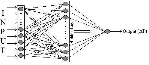 | Figure 1. Schematic diagram of the ANN |
 is the value of connection weight in the hidden layer then the weights are updated using the following equation during the epoch number
 ,
, | (1) |
 | (2) |
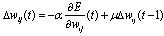
 represents the change of connection weights for the jth processing element in the hidden layer during epoch number t with that of ith input. a is learning rate and
  is the momentum coefficient.This is a second order learning algorithm that uses the method of optimization. If N is the number of epochs and n is the number of weights then the weight update equation is given as:
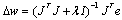 | (3) |
 Jacobian matrix and e is
  error matrix, I is the identity matrix and
  is the combination coefficient. In this algorithm the only user dependent parameter is
  , which is set only in the beginning. It is not required for the user to modify the value of
  during the training any more. When
  is large the algorithm becomes steepest descent and when it is small the algorithm becomes Gauss-Newton. In this way the Levenberg-Marquardt algorithm combines the best features of these two algorithms but avoids most of their limitations.This is a second order learning algorithm that uses the method of optimization. The SCG method is the advancement to that of the Conjugate Gradient (CG) method. In the Conjugate Gradient (CG) method the complexity of calculation for every epoch increases because of the line search to determine the correct step size, i.e., a line search requires several calculations of global error function or its derivative. In Scaled Conjugate Gradient (SCG) method there is no such line search required. It is fully automated and does not require the user to be involved during the training i.e., the user doesn’t have to provide some of the values of the user dependent parameters (like a ,
  etc. as mentioned above). This reduces the complexity significantly. This method uses the model-trust region approach known from Levenberg-Marquardt algorithm to scale the step size.
3.1. Performance of the ANN
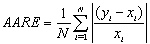
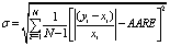
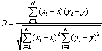
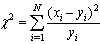
- The performance of the network is checked using the following parameters: Mean Squared Error (MSE),
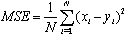 | (4) |
 | (5) |
 | (6) |
 | (7) |
 | (8) |
3.2. Optimization of the ANN
- Hidden layer(s) in ANN have the ability to deal very complex and nonlinear problems. Single hidden layer ANNs creates a hyper plane. The greater numbers of hidden layers improve the closeness-of-fit while a smaller number of hidden layers improve the smoothness or extrapolation capability of the ANN[54]. White[55] indicated that a hidden layer with arbitrarily large quantity of neurons can perform accurately, whereas Walczak[56] observed that a network containing two hidden layers perfom better than the single hidden layer network for specific problems. Bansal et al.[57] and Tamura and Tateishi[58] observed that the single hidden layer can solve most of the problems for more input variables and outputs. In the present case single hidden layer is used. In the hidden layer the numbers of processing elements are optimized by varying the number 1 to 25. Similar procedure was followed in our earlier studies by Bar et al.[47,48] and Bar and Das[51].The description of training procedure is elaborately described in our earlier paper[51]. Raw data are used as input variables without normalization. Initially the total data was randomized to prevent sampling error. Then 60% data points were used for training, 20% for cross-validation, 10% for testing and the rest used for prediction. Table 2 presents the four transfer functions used in the hidden layer. The output transfer function is given below,
 | (9) |
 | Figure 2. Variation of the minimum value of cross-validation MSE with the number of processing elements in the hidden layer for gas holdup for four different Transfer functions used in the hidden layer for BP algorithm in hidden and output layer |
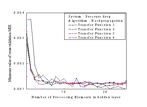 | Figure 3. Variation of the minimum value of cross-validation MSE with the number of processing elements in the hidden layer for pressure drop for four different Transfer functions used in the hidden layer for BP algorithm in hidden and output layer |
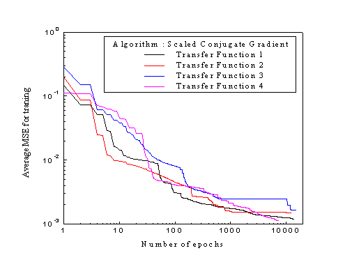 | Figure 4. Variation in the MSE for training using SCG algorithm vs. the numbers of epochs for the prediction of pressure drop |
|
| ||||||||||||||||||||||||||||||||||||||||||||||||||
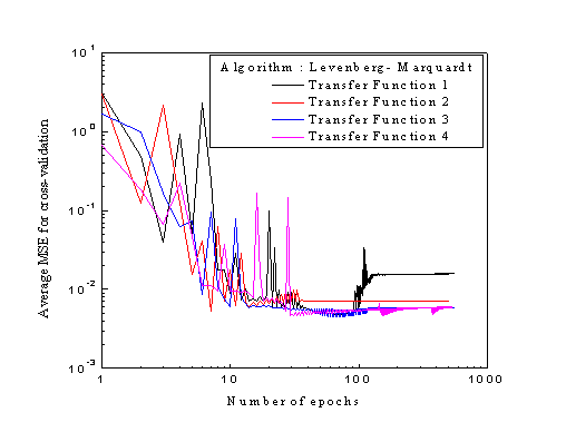 | Figure 5. Variation in the MSE for cross-validation using LM algorithm vs. the numbers of epochs for the prediction of pressure drop |
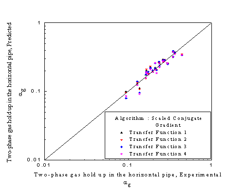 | Figure 6. Comparison of two-phase gas hold up across the horizontal tube for prediction using SCG algorithm in hidden and output layer with four different transfer function in the hidden layer for testing |
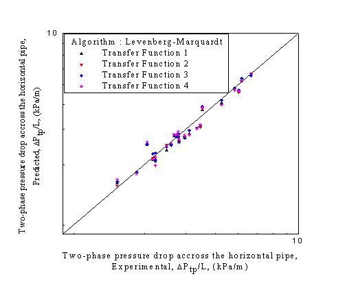 | Figure 7. Comparison of two-phase pressure drop across the horizontal tube for prediction using LM algorithm in hidden and output layer with four different transfer function in the hidden layer for testing |
| |||||||||||||||||||||||||||||||||||||||||||||||||||||||||||||||||||||||||||||||
| |||||||||||||||||||||||||||||||||||||||||||||||||||||||||||||||||||||||||||||||
 | Figure 8. Comparison of two-phase hold up across the vertical coil for prediction using LM algorithm in hidden and output layer with transfer function 1 in the hidden layer |
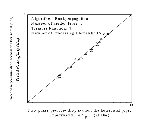 | Figure 9. Comparison of two-phase pressure drop across the vertical coil for prediction using BP algorithm in hidden and output layer with transfer function 4 in the hidden layer |
| |||||||||||||||||||||||||||||||||||||||||||||||||||||||||||||||||||||||||||||||||||||||||||||||
| |||||||||||||||||||||||||||||||||||||||||||||||||||||||||||||||||||||||||||||||||||||||||||||||
5. Conclusions
- A neural network based model was developed for the prediction of gas holdup and pressure drop for gas non-Newtonian liquid flow through horizontal pipe. A multilayer perceptron (one hidden layer) with three different algorithms namely Backpropagation, scaled conjugate gradient and Levenberg-Marquardt were used for this analysis. The ANN model accurately predicts the gas hold up and pressure drop across the horizontal pipe. The Chi-square test confirms that the best network for prediction of gas hold up is the transfer function 1 with 5 processing elements using Levenberg-Marquardt algorithm in the hidden and output layer. The Chi-square test also confirms that the best network for prediction of pressure drop is the transfer function 4 with 15 processing elements using Backpropagation algorithm in the hidden and output layer. Hence the developed ANN predictability should be useful in the scale-up of commercial pipeline.
References
| [1] | P. L. Spedding, and D R. Spence, “Prediction of Holdup in Two-Phase Flow,” Int. J Engg. Fluid Mech., vol. 1, pp. 67-82, 1988. |
| [2] | Wallis, G. B., One dimensional two-phase flow, McGrew-Hill Book Co. Inc., New York, 1969. |
| [3] | G. W. Govier, and K. Aziz, The Flow of Complex Mixtures in Pipes, Van Nostran Reinhold, New York City, 1972. |
| [4] | G. Hestroni, Handbook of Multiphase Systems, Hemisphere Publishing. Corp., Washington, DC, 1982. |
| [5] | C. T. Crowe, Multiphase Flow Handbook, CRC, 2006. |
| [6] | H. C. Ward, and J. M. Dallavalle, “Co-Current Turbulent–Turbulant Flow of Air and Water-Clay Suspensions in Horizontal Pipes,” Chem. Eng. Prog. Symp., vol. 10, pp. 1–14, 1954. |
| [7] | D. R. Oliver, and A. Young-Hoon, “Two-phase non-Newtonian flow, Part I: Pressure drop and holdup,” Trans. IChemE, vol. 46, pp. 106–115, 1968. |
| [8] | R. W. Lockhart, and R. C., Martinelli, “Proposed correlation of data for isothermal two-phase, two-component flow in pipes,” Chem. Engg. Progress, vol. 45, pp. 39–48, 1949. |
| [9] | R. G. Rosehart, E. Rhodes, and D. S. Scott, “Studies of gas-liquid (non-Newtonian) slug flow: void fraction meter, void fraction and slug characteristics,” Chem. Eng. J., 10(1), pp. 57–64, 1975. |
| [10] | R. Mahalingam, and M. A. Valle, “Momentum Transfer In Two-Phase Flow Of Gas-Pseudo-Plastic Liquid Mixtures,” Ind. Eng. Chem. Fundam. vol. 11, pp. 470–477, 1972. |
| [11] | R. G. Rosehart, D. Scott, and E. Rhodes, “Gas–liquid slug flow with drag-reducing polymer solutions,” AIChE J., vol. 18, pp. 744–750, 1972. |
| [12] | R. P. S. Srivastava, and G. S. R. Narasimhamurthy, “Hydrodynamics of non-Newtonian two-phase flow in pipes,” Chem. Eng. Sci., 28(2), 553–558, 1973. |
| [13] | R. P. S. Srivastava, and G. S. R. Narasimhamurthy, “Void Fraction and Flow Pattern during Two-Phase Flow of Pseudoplastic Fluids,” Chem. Eng. J., 21(2), 165–176, 1981. |
| [14] | K. P. Tyagi, and R. P. S. Srivastava, “Flow behavior of non-Newtonian liquid-air in annular flow,” Chem. Eng. J., 11(2), 147–152, 1976. |
| [15] | L. Otten, and A. S. Fayed, “Pressure drop and drag reduction in two-phase non-Newtonian slug flow,” Can. J. Chem. Eng., 54, 111–114, 1976. |
| [16] | L. Otten, and A. S. Fayed, “Slug Velocity and Slug Frequency Measurements in Concurrent Air/non-Newtonian Slug Flow,” Trans. Instn. Chem. Engrs., 55, 64–67, 1977. |
| [17] | N. I. Heywood, and J. F. Richardson, “ Head loss reduction by gas injection for highly shear-thinning suspensions in horizontal pipe flow,” Proc. Hydrotransport 5, Hanover, F. R. G., Paper C1, pp. 1–22, BHRA,1978. |
| [18] | S. I. Farooqi, N. I. Heywood, and J. F. Richardson, “Drag reduction by air injection for suspension flow in horizontal pipe line,” Trans. Instn. Chem. Engrs., 58, 16–27, 1980. |
| [19] | F. G. Eisenberg, and C. B. Weinberger, “Annular two-phase flow of gases and non-Newtonian liquids,” AIChE J., 25(2), 240–246, 1979. |
| [20] | N. Heywood, and M. E. Charles, “The Stratified Flow of Gas and non-Newtonian Liquid in Horizontal Pipes,” Int. J. Multiphase Flow, vol. 5, pp. 341–352, 1979. |
| [21] | S. I. Farooqi, and J. F. Richardson, “Horizontal flow of air and liquid (Newtonian and non-Newtonian) in a smooth pipe. Part I: A correlation for average liquid holdup,” Trans. IChemE, vol. 60, pp. 292–322, 1982. |
| [22] | S. I. Farooqi, and J. F. Richardson, “Horizontal Flow of air and liquid (Newtonian and non-Newtonian) in a smooth pipe. Part II: Average pressure drop,” Trans. IChemE, vol. 60, pp. 323–333, 1982. |
| [23] | R. P. Chhabra, S. I. Farooqi, J. F. Richardson, and A. P. Wardle, “Co-current flow of air and shear-thinning suspensions in pipes of large diameter,” Chem. Eng. Res. Des., vol. 61, pp. 56–61, 1983. |
| [24] | R. P. Chhabra, S. I. Farooqi, and J. F. Richardson, “Isothermal two-phase of air and aqueous polymer solutions in a smooth horizontal pipe,” Chem. Eng. Res. Des., vol. 62, pp. 22–31, 1984. |
| [25] | S. K. Das, M. N. Biswas, and A. K. Mitra, “Pressure Loses in Two-Phase Gas-Non-Newtonian Liquid Flow in Horizontal Tube,” J. Pipelines, vol. 7, pp. 307–325, 1989. |
| [26] | S. K. Das, M. N. Biswas, and A. K. Mitra, “Holdup for two-phase flow of gas-non-newtonian liquid mixtures in horizontal and vertical pipes,” Can. J. Chem. Eng., vol. 70, pp. 431–437, 1992. |
| [27] | M. Dziubinski, “A general correlation for the two-phase pressure drop in intermittent flow of gas and non-newtonian liquid mixtures in a pipe,” Trans. Chem. Eng. Res. Des., vol. 73, pp. 528–533, 1995. |
| [28] | D. Jinming, and Z. Jingxuan, “Studies on frictional pressure drop of gas-non-Newtonian fluid two-phase flow in the vacuum sewers,” Civil Engg. Environ. Systems, vol. 23, pp. 1–10, 2006. |
| [29] | M. J. Ruiz-Viera, M. A. Delgado, J. M. France, M. C. Sa´Nchez, and C. Gallegos, “On the drag reduction for the two-phase horizontal pipe flow of highly viscous non-newtonian liquid/air mixtures: Case of lubricating grease,” Int. J. Multiphase Flow, vol. 32, pp. 232–247, 2006. |
| [30] | J. Xu, Y. Wu, Z. Shi, L. Lao, and D. Li, “Studies on two-phase co-current air/non-Newtonian shear-thinning fluid flows in inclined smooth pipes,” Int. J. Multiphase Flow, vol. 33, pp. 948–969, 2007. |
| [31] | J. Xu, Y. Wu, D. Li, and H. Dong, “Effects of non-Newtonian liquid properties on pressure drop during horizontal gas-liquid flow,” J. Cent. South Univ. Technol., 14(s1), 112–115, 2007. |
| [32] | J. Xu, Y. Wu, H. Li, J. Guo, and Y. Chang, “Study of drag reduction by gas injection for power-law fluid flow in horizontal stratified and slug flow regimes,” Chem. Engg. J., vol. 147, pp. 235–244, 2009. |
| [33] | N. Jia, M. Gourma, and C. P. Thompson, “Non-Newtonian multi-phase flows: On drag reduction, pressure drop and liquid wall friction factor,” Chem. Engg. Sci., vol. 66, pp. 4742–4756, 2011. |
| [34] | R. Plippman, “An introduction to computing with neural nets,” IEEE ASSP Mag., vol. 4, pp. 4−22, 1987. |
| [35] | S. Cai, H. Toral, J. Qui, and J. S. Archer, “Neural network based objective flow regime identification in air-water two phase flow,” Can. J. Chem. Engg., vol. 72, pp. 440–445, 1994. |
| [36] | M. Leib, P. L. Mills, J. J. Lerou, and J. J. Turner, “Evaluation of neural networks for simulation of three-phase bubble column reactors,” Trans. IChemE, vol. 73, pp. 690–696, 1995. |
| [37] | Z. Bensetiti, F. Larachi, B. P. A. Grandjean, and G. Wild, “Liquid saturation in concurrent upflow fixed-bed reactors: a state-of-the-art correlation,” Chem. Engg. Sci., vol. 52, pp. 4239–4247, 1997. |
| [38] | F. Larachi, Z. Bensetiti, B. P. A. Grandjean, and G. Wild, “Two-phase frictional pressure drop in flooded-bed reactors: a state-of-the-art correlation,” Chem. Eng. Technol., vol.21, pp. 887–893, 1998. |
| [39] | S. Piche, F. Larachi, and B. P. A. Grandjean, “Improved Liquid Hold-up Correlation for Randomly Packed Towers,” Chem. Eng. Res. Des., vol. 79, pp. 71–80, 2001. |
| [40] | L. lliuta, B. P. A. Grandjean, and F. Larachi, “Hydrodynamics of trickle-flow reactors: updated slip functions for slit models,” Chem. Eng. Res. Des., vol. 80, pp. 195–200, 2002. |
| [41] | M.E. Shippen, and S.S.L. Scott, “A neural network model for prediction of liquid holdup in two-phase horizontal flow,” SPE 77499, Proc. SPE Annual Technical Conference and Exhibition, San Antonio, Texas, September – October, 2002. |
| [42] | E. A. Osman, and M. A. Aggour, “Artificial neural network model for accurate prediction of pressure drop in horizontal and near-horizontal-multiphase flow,” Pet. Sci. Technol., vol. 20, pp. 1–15, 2002. |
| [43] | M.R. Malayeri, H. M uller-Steinhagen, and J. M. Smith, “Neural network analysis of void fraction in air/water two-phase flows at elevated temperatures,” Chem. Engg. Sci., vol. 42, pp. 587–597, 2003. |
| [44] | A.Alizadehdakhel, M. Rahimi, J. Sanjari, and A. A. Alsairafi, “CFD and artificial neural network modeling of two-phase flow pressure drop,” Int. Commun. Heat Mass Transfer, vol. 36, pp. 850–856, 2009. |
| [45] | A. Shaikh, and M. Al-Dahhan, “Development of an artificial neural network correlation for prediction of overall gas holdup in bubble column reactors,” Chem. Engg. Proc., vol. 42, pp. 599–610, 2009. |
| [46] | S. Nasseh, A. Mohebbi, A. Sarrafi, and M. Taheri, “Estimation of pressure drop in venture scrubbers based on annular two-phase flow model, artificial neural networks and genetic algorithm,” vol. 150, pp. 131–138, 2009. |
| [47] | N. Bar, T. K. Bandyopadhyay, M. N. Biswas, and S. K. Das, “Prediction of Pressure Drop using Artificial Neural Network for non-Newtonian Liquid Flow through Piping Components,” J. Pet. Sci. Eng., vol. 71, pp. 187–194, 2010. |
| [48] | N. Bar, M. N. Biswas, and S. K. Das, “Prediction of Pressure Drop using Artificial Neural Network for Gas-non-Newtonian Liquid Flow through Piping Components,” Ind. Eng. Chem. Res., vol. 49, pp. 9423–9429, 2010. |
| [49] | N. Bar, M. N. Biswas, and S. K. Das, “Frictional Pressure Drop Prediction Using ANN for Gas-non-Newtonian Liquid Flow through 45° Bend,” Int. J. Artificial Intelligent Systems and Machine Learning, vol. 3, pp. 608–613, 2011. |
| [50] | S. Haykin, Neural networks – a comprehensive foundation, 2nd Ed. Prentice-Hall, USA, 1999. |
| [51] | N. Bar, and S. K. Das, “Comparative study of friction factor by prediction of frictional pressure drop per unit length using empirical correlation and ANN for gas-non-Newtonian liquid flow through 180° circular bend,” Int. Rev. Chem. Engg., vol. 3, pp. 628-643, 2011. |
| [52] | S. K. Das, (1988) “Studies on two-phase gas-non-Newtonian liquid flow in horizontal, vertical tubes and bends,” Ph.D. thesis, Dept. Chem. Engg., Indian Institute of Technology, Kharagpur, India. |
| [53] | B. Widrow, R. G. Winter, and R. A. Baxter, “Layered Neural Nets for Pattern Recognition,” IEEE Trans. Acoustics, Speech and Signal Processing,” vol. 36, pp. 1109–1118, 1988. |
| [54] | E. Barnard, and L. Wessels, “Extrapolation and interpolation in neural network classifiers,” IEEE Control Systems, vol. 12, pp. 50–53, 1992. |
| [55] | H. White, “Connectionist nonparametric regression: multilayer feed-forward networks can learn arbitrary mapping,” Neural Networks, vol. 3, pp. 535–549, 1990. |
| [56] | S. Walczak, “Developing neural nets currency trading,” Artificial Intelligence in Finance, vol. 2, pp. 27–34, 1995. |
| [57] | A. Bansal, R. J. Kanuffman, and R. R. Weitz, “Comparing the modeling performance of regression and neural networks as data quality varies: a buisnessvalue approach,” J. Manag. Information Systems, vol. 10, pp. 11–32, 1993. |
| [58] | S. Tamura, and M. Tateishi, “Capabilities of four layered feedforward neural network: four layers versus three,” IEEE Trans. Neural Net., vol. 8, pp. 251–255, 1997. |