1. Introduction

The coasts of Louisiana and other southeastern US states are highly susceptible to storm events, along with their accompanying precipitation, which result in frequent flooding of urban areas [3]. There are various storm impacts to the shoreline and storm impacts affecting human activities located in this region [14]. These storm events can increase the potential for enteric pathogenic contamination in surface waters through combined sewer overflows and agricultural runoff [20]. This threat is growing as the region continues to urbanize. Exposure to Fecal Indicator Bacteria (FIB) contaminants has been linked to Gastrointestinal Illness (GI), [3], and deaths due to Vibrio vulnificus infections have been documented during past disasters such as Hurricanes Katrina and Harvey [21]. Measuring the concentration of Fecal Indicator Bacteria (FIB) during major storm events can help inform management and response actions. However, microbial analysis for FIB through lab-based methods typically requires a 24-hour processing time [17] and is costly. Waiting for the results of lab-based methods does not provide enough time to estimate FIB and the potential risks of population exposure to FIB. The nowcasting approach we present provides FIB estimates, based on historical data, and provides a tool to obtain rapid estimates during storm events.

Statistical modeling techniques, such as Multiple Linear Regression (MLR), ([9]; [6]; [18]), Artificial Neural Networks (ANN), ([26]; [13]; [16]), and Machine Learning (ML), ([4]; [1]; [23]), have been used to rapidly ‘nowcast’ (estimate/predict the current or near-term state using real-time data and predictive analytics) FIB based on other environmental parameters (e.g., water temperature, dissolved oxygen, turbidity, specific conductivity, precipitation, average wind speed, current [parallel to shore and perpendicular to shore], etc.), allowing an immediate response to warn communities of contamination risks [25] A number of studies have assessed FIB using MLR, ANN, and ML methods. However, the focus of those studies was not on the impact of FIB on the Gulf Coast region of the United States. US EPA has recommended using two FIB, Enterococci and Escherichia coli (E. coli), as indicators of fecal contamination [24]. Enterococci and E. coli are better indicators of fecal contamination than the previously used indicators of total coliforms and fecal coliforms [24]. Enterococci are good predictors of GI in both marine and fresh recreational waters, while E. coli are good predictors of GI in fresh water only [24].

Since enterococci is an indicator of fecal contamination in both marine water and fresh water, it was selected as the FIB for this study. In this study, we seek to: a) create a model to accurately nowcast enterococci concentrations from other environmental/water quality parameters at selected study sites; b) determine if a model that predicts enterococci concentration under “normal” or baseline conditions can be applied to do the same during storm events, and; c) determine how well such a model, trained on recent historical data, will predict the probability of exceedances/non-exceedances of FIB (enterococci) concentrations and concentration accuracies at extreme high/low values. Our scoping study provides a way to select between optimized statistical models to enhance our understanding of the key factors (i.e., measured independent variables {IVs}) influencing bacterial concentrations (FIB) during storm events. The measured IVs in this study are the water quality and weather parameters that were sampled at six sites around Lake Pontchartrain and include the following: water temperature (°C), dissolved oxygen (mg/L), specific conductivity (microsiemens per centimeter [µS/cm]), salinity (parts per thousand), turbidity (Nephelometric Turbidity Units [NTUs]), ambient (air) temperature (°C), pH, cumulative 72-hour precipitation (prior to sampling), average wind, along shore current, offshore current, and FIB {E Coli, Fecal Coliform, and Enterococci}. The response (dependent) variable is the predicted FIB (enterococci).

We used data from six Lake Pontchartrain sampling sites, selected from three rural sites on the north side of the lake (Sites 8, 9, and 10), along with three urban sites on the south side of the lake (Sites 2, 3, and 4) to develop models for predicting the amount of Fecal Indicator Bacteria (FIB) that could be expected in those recreational waters after storm events in the area. These six sites were selected because the primary use of the water at those sites is recreational, and those sites would be representative of where people spent time in the water and could come in contact with FIB. The weather conditions were measured at 3 weather stations and 1 NOAA weather buoy located around Lake Pontchartrain. The local airport weather stations closest to each of the six sampling sites around Lake Pontchartrain, used to determine weather conditions at the six sites, are as follows: Site 2 – New Orleans Louisiana (NOLA) Airport (Weather Station: USW00012916), Site 3 and Site 4 – Lakefront Airport (Weather Station: USW00053917), Site 8, Site 9, and Site 10 – Slidell Airport (Weather Station: USW00053865). The NOAA weather buoy located in Lake Pontchartrain provides very precise wind data. The weather conditions that were monitored at the three weather stations include the following: precipitation, wind direction, wind gust (m/s), wind speed (m/s), water temperature (°C), ambient (air) temperature (°C, wave height (m), barometric pressure (hPa), dew point (°C), visibility (mi), and tide (height: ft).

2. Materials and Methods

2.1. Study Area

For our study area, shown in Figure 1, we focused on Lake Pontchartrain, a large estuary north of New Orleans, LA. The Pontchartrain Conservancy, a local nonprofit group, has collected weekly measurements of enterococci concentration and other water quality parameters at 15 recreational beaches and boat launch sites (two of the 15 sites have been decommissioned) around the estuary since 2001. We selected data from 6 sampling sites to compare urban and rural FIB: 3 sites (Site #2, Site #3, and Site #4) are located on Lake Pontchartrain’s highly urbanized southern shore recreational beaches near New Orleans (blue circles in Figure 1), and 3 sites (Site #8, Site #9, and Site #10) are located on Lake Pontchartrain’s more rural northern shore recreational beaches in St. Tammany Parish, LA (red circles in Figure 1). We combined these water quality observations with weather data including wind speed, wind direction, water temperature, and precipitation, etc., obtained from 3 National Oceanic and Atmospheric Administration (NOAA) weather stations (three orange boxes in Figure 1) and a new NOAA weather buoy near the Lake Pontchartrain’s south shore (single black box in Figure 1).

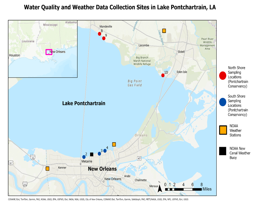Figure 1. Water Quality Measurement and Weather Data Collection Sites around Lake Pontchartrain, LA

2.2. Determining Study Area Wind and Shore Configuration

VB₃ calculated wind components parallel and perpendicular to shore at each site based on the angle of the shoreline using the following formulas (Cyterski et al., 2019):

(1)

(2)

Where S is wind speed, D is wind direction, B is the beach orientation in degrees with respect to the water (see Figure 2 and Figure 3) and π ≈ 3.1416. Figure 2 displays the general orientation of the land with respect to the water and Figure 3 displays beach orientation.

The map control function in VB₃ permits the user to define the boundaries of a beach so that VB₃ can calculate beach orientation [7]. This capability is important if wind, wave, and/or current flow components are used in building the model(s). Wind components and beach orientation can be powerful predictors of pathogen indicator concentrations at a beach [7]. Defining the beach orientation is recommended if the beach dataset being analyzed has wind, current, or wave data. We incorporated the wind speed and direction data, determined using Figure 2 and Figure 3 orientations along with the water quality and weather observations for each site. The (South Shore) beach orientation for Sites 2, 3, and 4, and (North Shore) beach orientation for Sites 8, 9, and 10 were calculated using the VB₃ mapping interface to determine the site angles for each of the sites. The A and O were calculated for each site using data in an Excel-compatible comma-separated value (*.csv) file (NOAABuoy_2015_2022.csv). For each site observation, we included the total (cumulative) precipitation, measured at the weather station nearest to each site in the 72 hours prior to enterococci sampling.

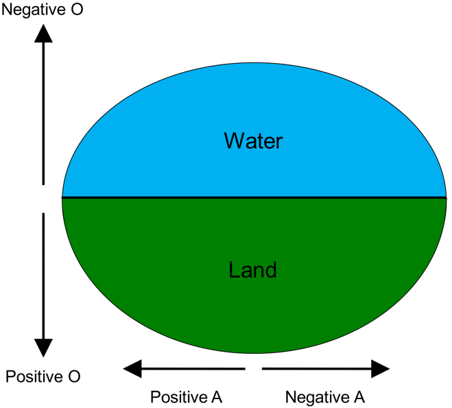Figure 2. Coordinate System for Measuring Alongshore Wind (A) and Offshore Wind (O) Positive and Negative Components [7]

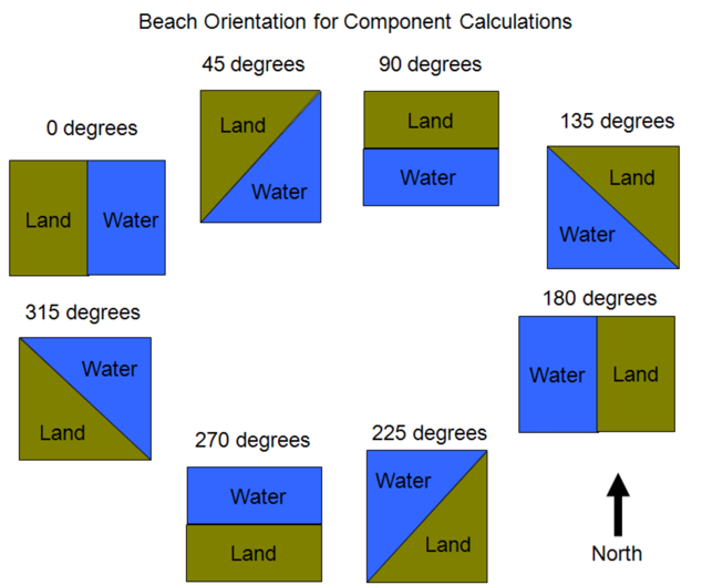Figure 3. Orientation of Beach (site positioning) with Respect to Water [7]

2.3. VB₃ Models Used (MLR and GBM)

When applying models (i.e., MLR, GBM) to a dataset, VB₃ calculates an Analysis of Variance (ANOVA) to assess the overall significance of a model's ability to explain the variation in the response variable (e.g., enterococci levels) based on the independent variables (e.g., precipitation, temperature, turbidity, etc.). The ANOVA result from VB₃ produces a P-value, which represents the probability of observing the differences in means between the groups (or the relationships between variables in the model) by random chance, assuming the null hypothesis (no relationship or difference between means). We trained our models using data from 2015-2022 (1811 total observations, ~300 per site: for training and cross validation) and from 2023-2024 (577 total observations, ~96 per site: testing dataset).

2.4. BSTS Model (Independent from VB₃)

We developed and applied a BSTS model to the 3 sites (Site #2, Site #3, and Site #4) on Lake Pontchartrain’s southern shore and the 3 sites (Site #8, Site #9, and Site #10) on Lake Pontchartrain’s northern shore. The log-transformed enterococci concentration was the response variable for the six sites. Each site had its own BSTS model to capture the unique environmental and observational characteristics of each site. From a processing perspective, the BSTS model is divided into an observation equation and four state equations for each site. The observation equation consists of the observed log-transformed enterococci concentration at each site, and the state equation (latent state) at each specified time for each site. The BSTS method explicitly includes the temporal structure/time-dependency of the data as opposed to the GBM and MLR approaches.

The state equation (latent state) for each site consists of four components: a) the level [baseline value or central tendency of the time series data]; b) the trend [direction or rate of change of the time series data over time]; c) seasonal components [seasonal periodicity of the time series data], and; d) predictor effects [captures influence of external regressors]. The regression component of the BSTS model includes the effects of external predictors on each site’s time series. The BSTS external predictors were selected based on the results of the VB₃ GBM model so that the most influential variables were incorporated into the BSTS analysis. The BSTS model used station-dependent predictors with each station having its own tailored set.

The observed time series data used in the BSTS model covers the September 2015 to December 2024 time period. In developing the BSTS model, the data from September 2015 to December 2022 was used to ‘train’ the model. The data for the year 2023 was used to validate and update the BSTS model, while the 2024 data was used to test the model. The training data set (September 2015 to December 2022) was used to help the model ‘learn’ historical patterns and trends, and the validation set (2023) was used fine-tune the model parameters and components so that it adapted to changes without overfitting the model. The test set (2024) was used to provide an unbiased evaluation of the model’s predictions on future data and confirm its robustness and generalizability.

3. Results

3.1. VB₃ (GBM)

We generated GBM models in VB₃ with log10(Enterococci) as the response variable/Decision Threshold (DC) to determining exceedance compared to log₁₀(33 CFU/100mL as the Regulatory Standard (RS) [24], setting the seed value to 1. When a GBM model is generated, VB₃ displays a table showing the percent (%) influence of each independent variable in the model, as shown in Table 1, as well as a table showing the GBM model’s sensitivity, specificity, accuracy, true/false positives, and true/false negatives that are calculated using five-fold cross validation (Table 2). For GBM models in VB₃, an independent variable’s influence is the percentage of branches across all of the decision trees including that variable (i.e., the most influential independent variables are those that are used most often to create the decision tree branches). There is a tradeoff between sensitivity and accuracy of the models, and VB₃ allows the user to adjust the decision threshold to find an appropriate balance between sensitivity and accuracy. We adjusted the threshold to give the highest possible sensitivity, while maintaining an accuracy of at least 70% (or as close to 70% as possible). After documenting the results, we removed the independent variable with the least influence (bringing the number of independent variables from 8 to 7), generated a new model, and adjusted the threshold to balance sensitivity and accuracy. We repeated this process until we arrived at a model in which every independent variable had at least a 10% influence. We then compared the sensitivity, specificity, and accuracy values of the models (one with 8 variables, one with 7 variables, and so on) and selected the one that gave the highest accuracy and highest sensitivity while using as few variables as possible, as shown in Table 1.

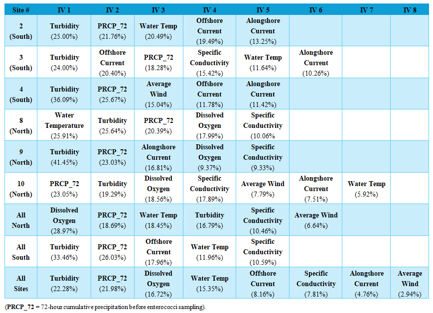Table 1. VB3 GBM Results for Independent Variables (IVs) Ranked from Greatest to Least Influence at: a) Individual Sites, b) North Sites, c) South Sites, d) All Sites

3.2. Most Influential Independent Variables

The independent variables (IVs) in Table 1 are arranged in order from the most influential IVs to the least influential IVs in estimating enterococci concentrations. When viewing Table 1, the GBM models generated in VB₃ demonstrate that, based on the collected sampling/measurement data, the two most influential IVs for estimating/modeling enterococci concentrations are turbidity and cumulative 72-hour precipitation (prior to sampling). This is true for 4 of the 6 sampling locations (Site 2 and Site 4 [South Shore], along with Site 9 and Site 10 [North Shore]). The VB₃ GBM model that incorporates all 6 sites (All Sites) and the VB₃ GBM model that incorporates all South Shore sites (All South) also show that the two most influential independent variables (IVs) for estimating /modeling enterococci concentrations are turbidity and cumulative 72-hour precipitation (prior to sampling).

A total of 6 of the 9 VB₃ GBM models illustrated in Table 1 indicate that the two most influential independent variables (IVs) for estimating/modeling enterococci concentrations are turbidity and cumulative 72-hour precipitation (prior to sampling). The GBM model for Site 3 has turbidity as the most influential IV and cumulative 72-hour precipitation (prior to sampling) as the third-most influential IV for estimating/modeling enterococci concentrations. The GBM model for Site 8 has turbidity as the second most influential IV and cumulative 72-hour precipitation (prior to sampling) as the third-most influential IV for estimating/modeling enterococci concentrations. The GBM model that incorporates all North Shore sites (All North) has cumulative 72-hour precipitation (prior to sampling) as the second-most influential IV and turbidity as the fourth most influential IV for estimating/modeling enterococci concentrations.

This aligns with investigations that have shown that higher turbidity increases enterococci survival in the environment by limiting their exposure to UV radiation [5], and runoff from rainfall is linked to increased enterococci in rivers [8]. Increased turbidity increases enterococci concentration because: a) resuspended sediment releases trapped bacteria into the water; b) sediment particles shields the bacteria from UV radiation which generally kills the bacteria, and; c) sediment particles provide growth-sustaining nutrients to bacteria. Increased precipitation causes increased turbidity through soil erosion and washes fresh bacteria into waterways. Other studies did not include cumulative 72-hour precipitation (prior to FIB sampling) as a predictor of enterococci concentration. Although median enterococci concentrations generally met the EPA’s 2012 recommended recreational water quality criteria for freshwater log₁₀ (33 CFU/100 mL), exceedances were observed 45% of the time [24]. Sampling site number 8 (1^st ‘box and whiskers’ plot on the right-hand side of Figure 4) exceeded the recommended criteria level 68% of the time, as shown in Figure 4. This might be explained by the fact that Site 8 tends to have higher enterococci concentration measurements as compared to the site closest to it geographically (Site 9). The Bayesian Structural Time-Series (BSTS) model observed log-transformed enterococci versus predicted plots indicate that the predicted values generally follow the trends of the observed values.

To determine if there was a turbidity threshold at which major changes in enterococci occurred, the observations were divided into three levels (<10 NTU, between 10 and 50 NTU, and >= 50 NTU) based on the Bonferroni-corrected ANOVA analysis, as shown in Figure 5. The Bonferroni-corrected ANOVA was used to determine if there was a statistically significant difference in enterococci between the three levels. We conducted this analysis separately for each sampling site. Our analysis indicated a significant difference in enterococci concentrations between all turbidity levels. In Table 3, we see that the enterococci concentrations as a function of turbidity are unlikely to have occurred by chance (P<0.05). Enterococci exceeded recommended criteria levels when turbidity was >50 NTU, as shown in Figure 4.

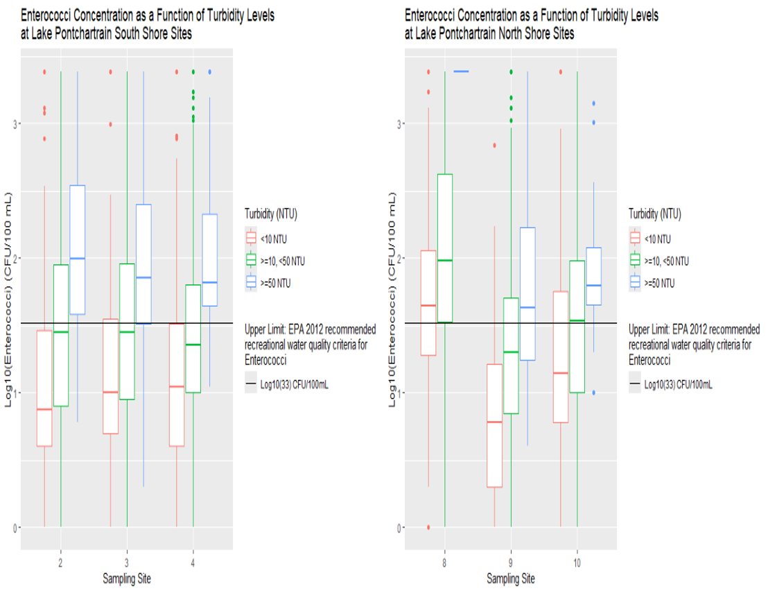Figure 4. Enterococci Concentration as a Function of Turbidity Levels at Lake Pontchartrain South Shore Sites (Sites 2, 3, and 4) versus North Shore Sites (Sites 8, 9, and 10). The black horizontal line indicates the upper limit of the EPA’s 2012 recommended recreational water quality criteria for enterococci in freshwater

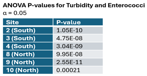Table 2. Enterococci Concentration as a Function of Turbidity Levels with ANOVA P-values at Lake Pontchartrain South Shore Sites (Sites 2, 3, and 4) and North Shore Sites (Sites 8, 9, and 10). The low P-values indicate that the enterococci concentrations as a function of turbidity are unlikely to have occurred by chance

Figure 5 displays the turbidity measured at each sampling site compared to the EPA’s 2012 recommended recreational water quality criteria for enterococci in freshwater. This indicates that higher enterococci concentrations seem to correlate with higher levels of turbidity. Higher turbidity indicates the presence of an increased number of suspended particles in the water, which is associated with increased bacterial growth and higher enterococci concentrations. We conducted the same Bonferroni-corrected ANOVA analysis with 72-hour cumulative precipitation (prior to FIB sampling), which divided precipitation into 3 levels (<0.5 in, between 0.5 and 2 in, and >= 2 in), as shown in Figure 6. We found that 72-hour cumulative precipitation which totaled >0.5 inches significantly increased enterococci concentrations when compared to concentrations at <0.5 inches of rain. We conducted this analysis separately for each sampling site. In Table 4, we see that the enterococci concentrations as a function of 72-hour cumulative precipitation levels (prior to FIB sampling) are unlikely to have occurred by chance given the statistical significance (P<0.05).

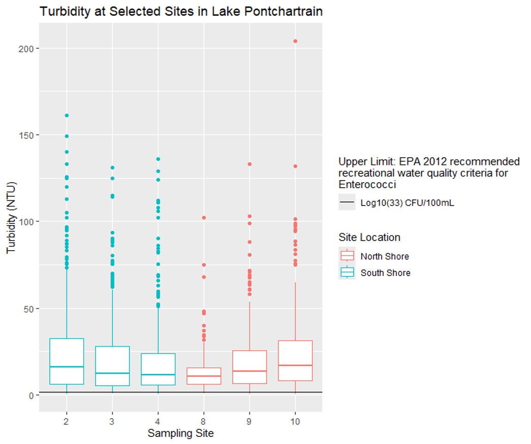Figure 5. Measured Turbidity at Sampling Site. The black horizontal line indicates the upper limit of the EPA’s 2012 recommended recreational water quality criteria for enterococci in freshwater

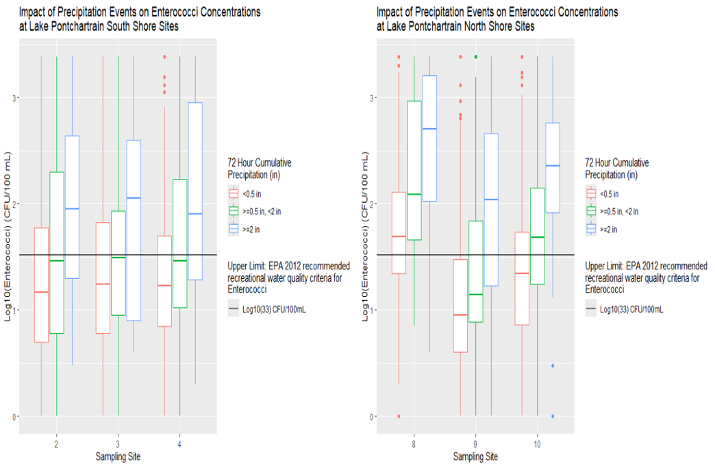Figure 6. Impact of 72-Hour Cumulative Precipitation Events on Enterococci Concentration at Lake Pontchartrain South Shore Sites (Sites 2, 3, and 4) versus North Shore Sites (Sites 8, 9, and 10). The low P-values indicate that the enterococci concentrations as a function of 72-hour cumulative precipitation are unlikely to have occurred by chance. The black horizontal line indicates the upper limit of the EPA’s 2012 recommended recreational water quality criteria for enterococci in freshwater

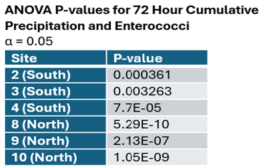Table 3. Enterococci Concentration as a Function of 72-Hour Cumulative Precipitation Levels with ANOVA P-values at Lake Pontchartrain South Shore Sites (Sites 2, 3, and 4) and North Shore Sites (Sites 8, 9, and 10). The low P-values indicate that the enterococci concentrations as a function of 72-hour cumulative precipitation are unlikely to have occurred by chance

We observed that enterococci concentrations increased in the days following storms with significant rainfall, then returned to initial (background) levels approximately 2 weeks after a storm event. While the predicted enterococci concentration values from the VB₃ GBM models captured overall trends in observed enterococci concentration and accurately predicted exceedances or non-exceedances of the EPA’s 2012 recommended recreational water quality criteria for enterococci in freshwater, they underpredicted extremely high and extremely low values, as shown in Figure 7 and Figure 8, where red represents the modeled values and black represents the observed values. A representative South Shore Site (Site 2) and a representative North Shore Site (Site 9) were selected to illustrate the underprediction of high and low values by the GBM. This an issue that has been documented with GBM methods in other studies ([28]; [10]).

Figure 7 and Figure 8 compare the observed enterococci concentration values to those predicted by the GBM model. The GBM model in VB₃, as displayed in Figure 7 and Figure 8, tends to underpredict the extreme values (both high and low) of the enterococci concentrations. This is common to GBM models, and perhaps this can be attributed to the fact that GBMs are susceptible to overfitting and are designed as an optimization function created to minimize a loss function.

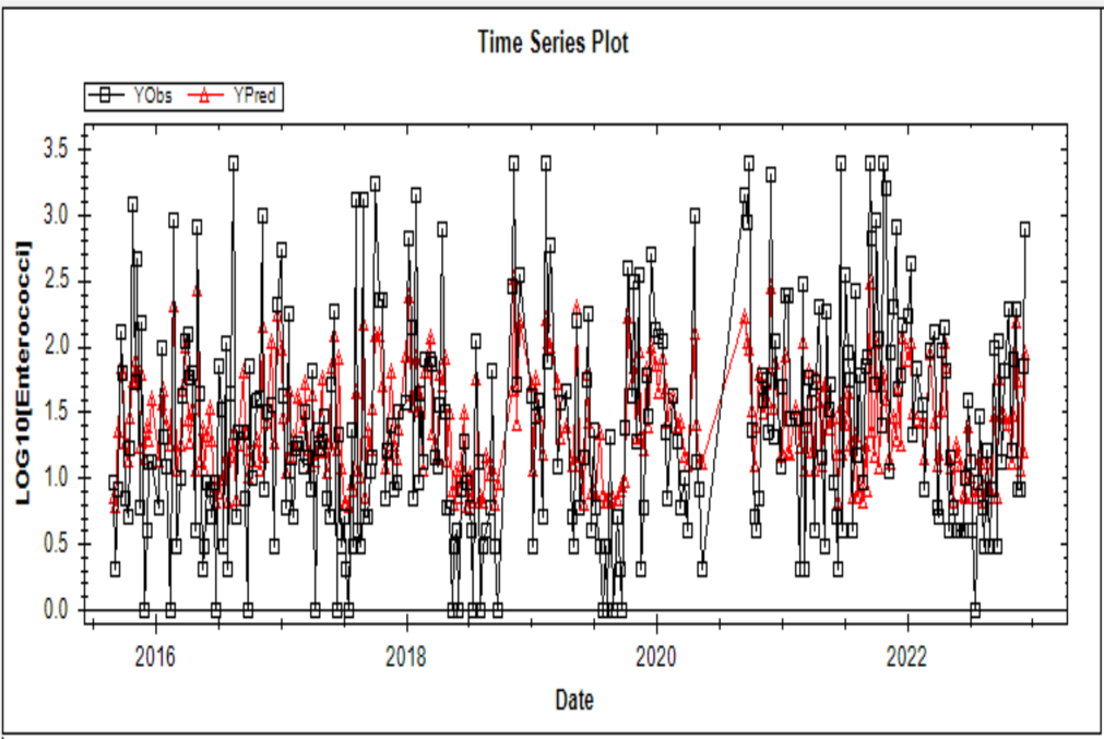Figure 7. Fitted vs. Observed Enterococci Concentrations (Log10 Normalized) at Site 2 (South Shore) from VB3 GBM Model

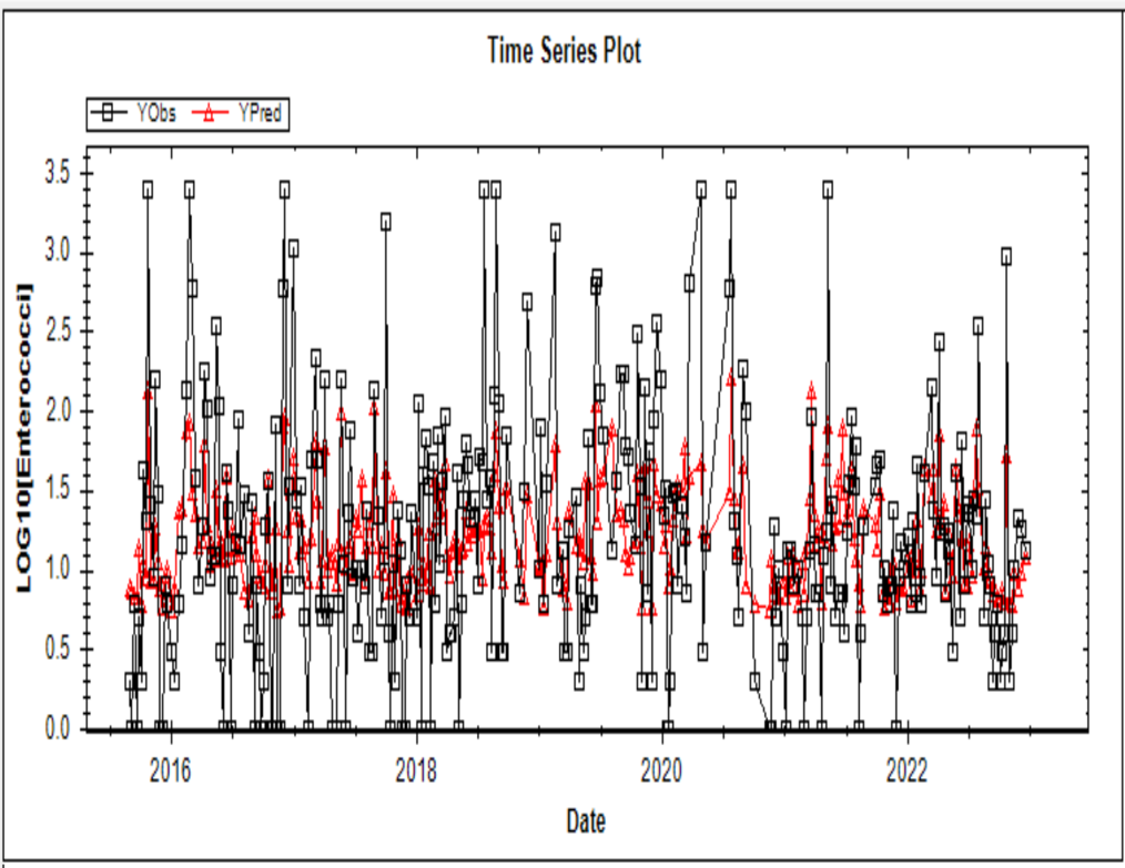Figure 8. Fitted vs. Observed Enterococci Concentrations (Log10 Normalized) at Site 9 (South Shore) from VB3 GBM Model

3.3. GBM Model Cross-Validation

Cross-validation in VB₃ GBM models allows the assessment of real-world prediction accuracy. GBM model selection is accomplished based on the true positive (TP), true negative (TN), false positive (FP), and false negative (FN) counts, that are calculated by 5-fold cross validation. The data are split randomly and evenly into five subsets, and five models are built to predict exceedances on each of the five subsets. For each of these models, the predicted subset is left out of model building, so the TP, TN, FP, and FN counts reflect prediction of novel observations, not the accuracy in fitting past observations. In contrast, MLR model performance in VB₃ is based on fitted results and not cross-validated results.

Performing cross-validation in VB₃ allows the user to set two parameters for each model, the sample size for the testing data and the number of random samples taken. In VB₃ cross-validation, a random sample of the user-selected sample size is taken from the modeling dataset and kept for later use. Each “Best Fits” model is then ‘refit’ to the remaining training data. The independent variables in each model remain the same, but the regression coefficients are adjusted to reflect the least-squares fit to the training data.

The Mean Squared Error of Prediction (MSEP) is then calculated based on the sample size for the testing data for each candidate model. This process is done for the number of random samples taken. A table then displays the average MSEP values for each of the 10 “Best-Fit” models.

Cross-validation allows evaluation of which candidate model consistently makes the best predictions, i.e., has the lowest MSEP. The recommendation for VB₃ is that approximately 25% of the total number of observations be used for testing, and that at least 1000 trials be performed. The cross-validation is performed to ensure that predictions on future data points are nearly as good as the model fits. GBM model accuracy values calculated from cross validation of the VB₃ for this analysis were roughly 0.7 (ranging from 0.67 to 0.74), with sensitivity values ranging from 0.72 to 0.85, and specificity values ranging from 0.5 to 0.73, as shown in Table 4 below. In VB₃, we used the corrected Akaike Information Criterion (AICc) as the model evaluation criteria to assess model fitness. The Decision Criteria (DC), and the Regulatory Standard (RS) are used to set the level of where exceedance/non-exceedance is determined {i.e., log10(Enterococci) = log₁₀(33 CFU/100mL)} and have the same units. The DC and RS allow model sensitivity, specificity, and accuracy to be determined, and the number of true/false positives, and true/false negatives to be calculated. The results are based on the cross-validation of the training data.

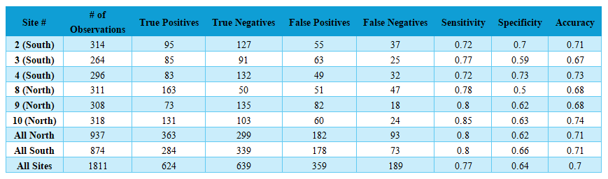Table 4. VB3 GBM Model Cross-Validation Results (All Sites)

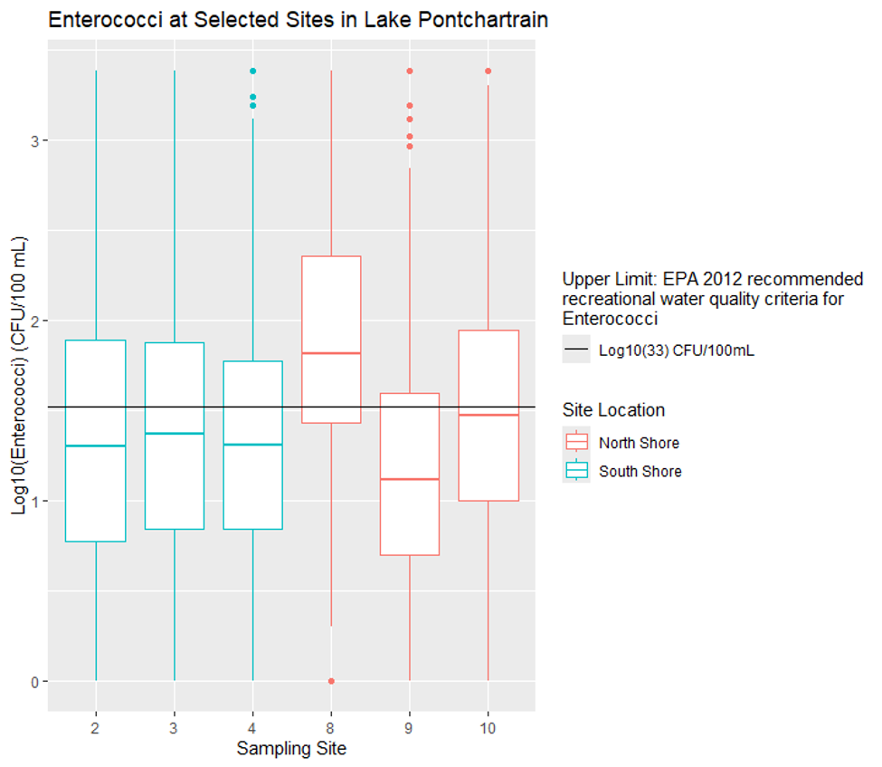Figure 9. Enterococci Concentration Measurements at Sites on Lake Pontchartrain. The black horizontal line indicates the upper limit of the EPA’s 2012 recommended recreational water quality criteria for enterococci in freshwater

3.4. MLR Analysis

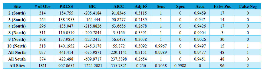
In VB₃, the MLR analysis was implemented using the following process: a) all independent variables were selected (same as for the GBM analysis); b) the genetic algorithm was selected; c) the seed value was set to 1; d) use AICc as the model selection criteria; e) run VB₃ and select each of the best fit models; f) use cross-validation for the selected models; g) select 10% of observations and run 1000 tests; h) use BIC as the model selection criteria and repeat steps e), f) and g); i) use PRESS as the model selection criteria and repeat steps e), f) and g). Note that MLR model performance is based on fitted and not cross-validated results in VB₃.

Table 5. VB3 MLR Model Results (All Sites)

3.5. BSTS Analysis

For the BSTS model analysis, the actual observed log-transformed enterococci concentration values versus the predicted values were plotted for the Jan 2023 – Jan 2024 time period (Figures 10 – 12) and for Jan 2024 – Dec 2024 (Figures 13 – 15). The overall pattern displayed for these plots (Jan 2023 – Jan 2024) is that the predicted values tend to follow the general trend of the observed values with only a few predicted values exceeding the maximum or minimum observed log-transformed enterococci concentration values. The overall pattern for the Jan 2024 – Dec 2024 plots is that there are some exceedances of the minimum observed log-transformed enterococci concentration values.

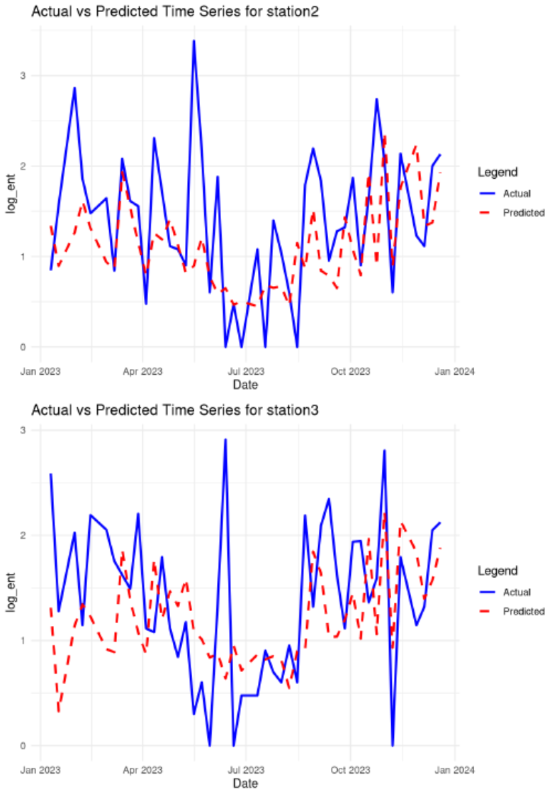Figure 10. Actual vs. Predicted Enterococci Concentrations (Log10 Normalized) at Site 2 and Site 3 (South Shore) from BSTS Model: Jan 2023 – Jan 2024

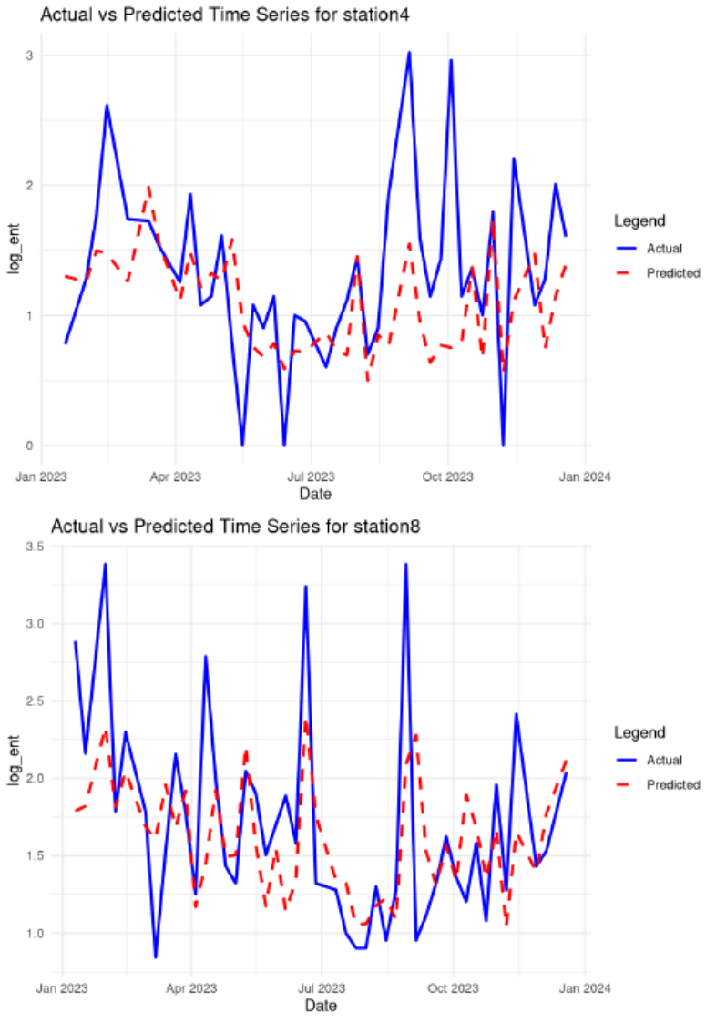Figure 11. Actual vs. Predicted Enterococci Concentrations (Log10 Normalized) at Site 4 (South Shore) and Site 8 (North Shore) from BSTS Model: Jan 2023 – Jan 2024

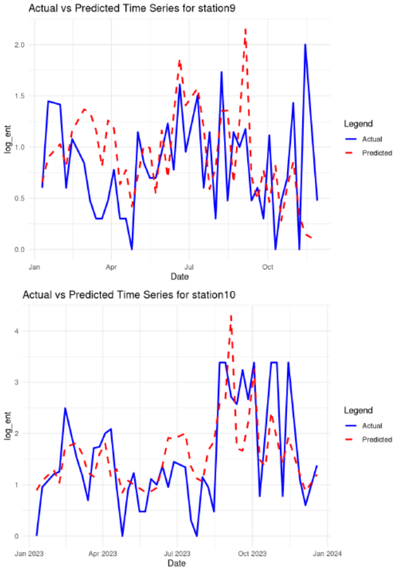Figure 12. Actual vs. Predicted Enterococci Concentrations (Log10 Normalized) at Site 9 and Site 10 (Norh Shore) from BSTS Model: Jan 2023 – Jan 2024

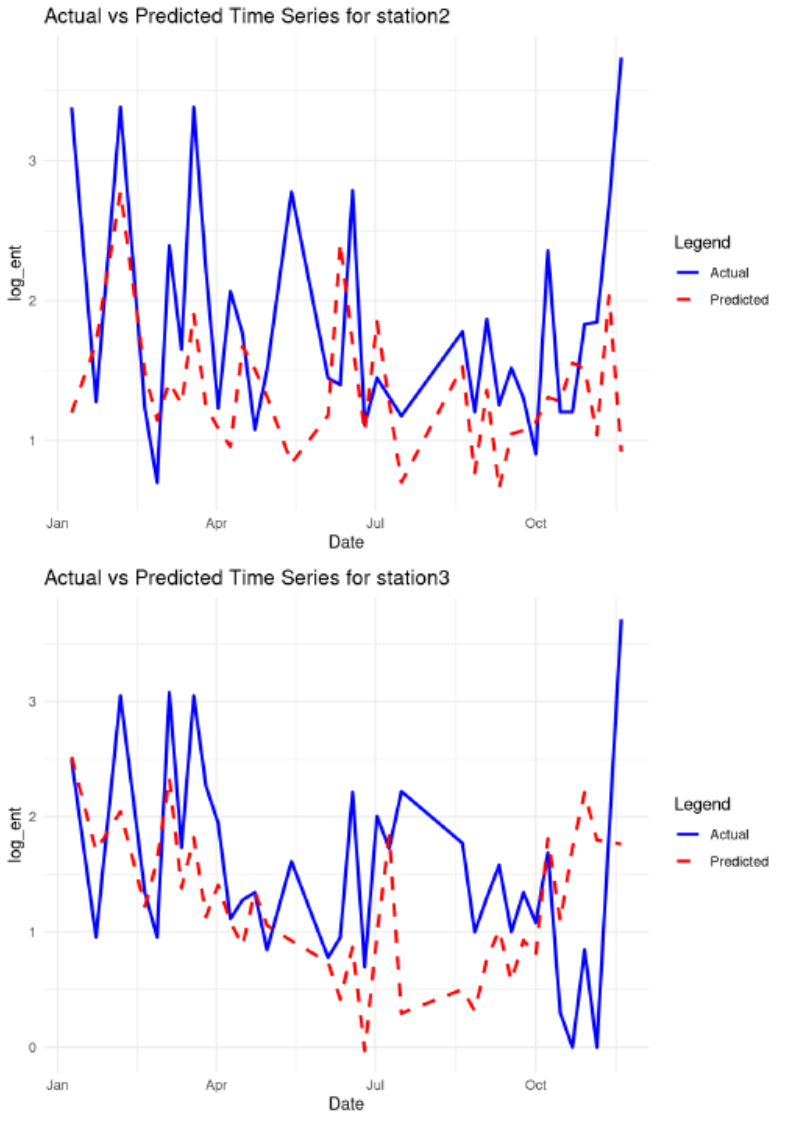Figure 13. Actual vs. Predicted Enterococci Concentrations (Log10 Normalized) at Site 2 and Site 3 (South Shore) from BSTS Model: Jan 2024 – Dec 2024. There were no observations for Site 4 in 2024

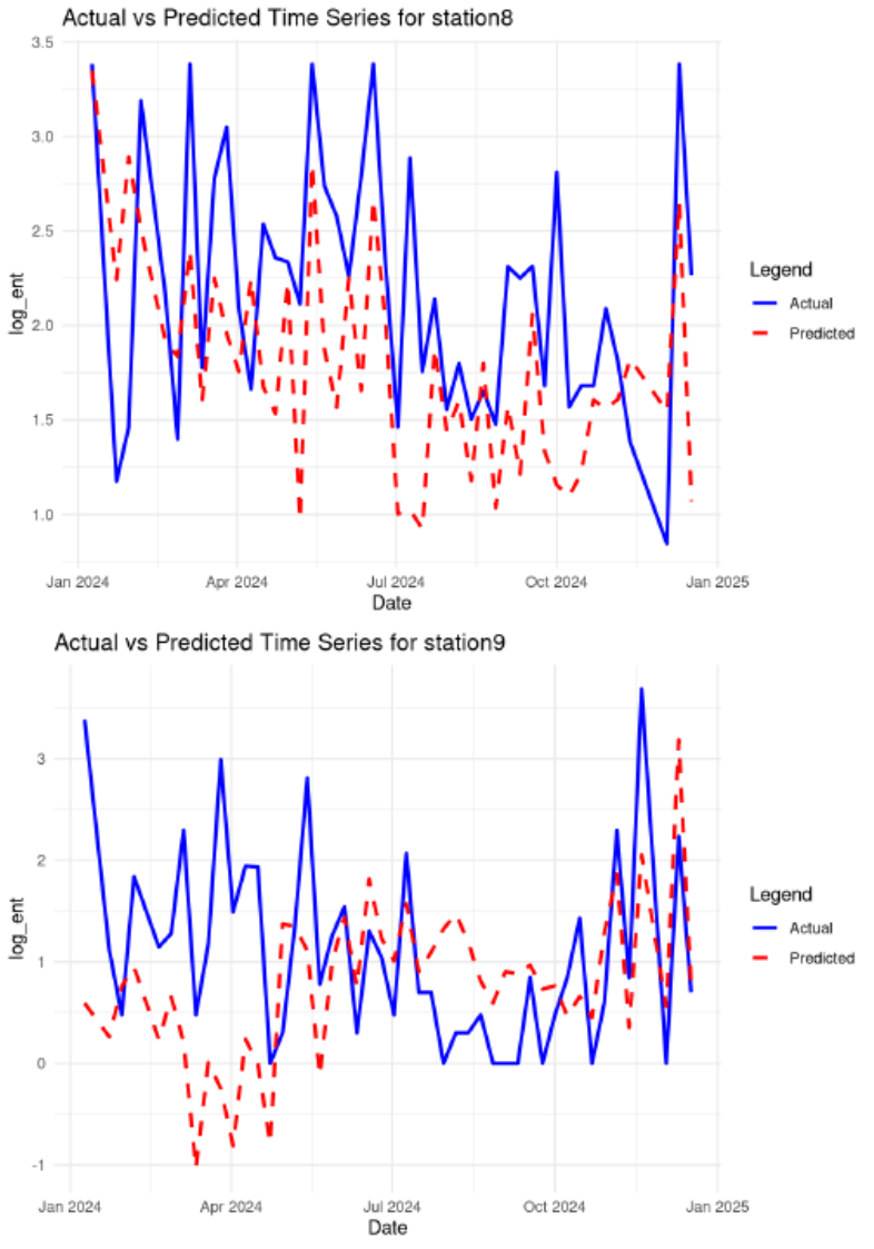Figure 14. Actual vs. Predicted Enterococci Concentrations (Log10 Normalized) at Site 8 and Site 9 (North Shore) from BSTS Model: Jan 2024 – Dec 2024

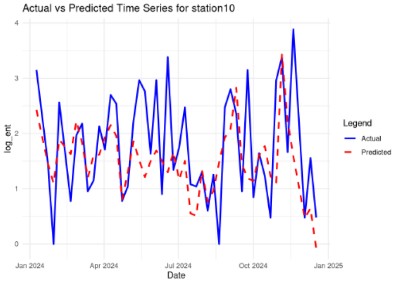Figure 15. Actual vs. Predicted Enterococci Concentrations (Log10 Normalized) at Site 10 (North Shore) from BSTS Model: Jan 2024 – Dec 2024

4. Discussion

We developed predictions for enterococci concentrations using the Multiple Linear Regression (MLR) in VB₃, and Generalized Boosted Regression Modeling (GBM) models in VB₃, and a Bayesian Structural Time Series (BSTS) model, developed and applied independently of VB₃, to the weekly water quality data from Lake Pontchartrain to analyze our water quality parameter and weather datasets. The objective of this analysis was to determine if we could develop model estimates to identify and predict exceedances of the EPA’s 2012 recommended recreational water quality criteria for enterococci in freshwater (log₁₀ [33 CFU/100 ml]). We used the water quality and weather data from Lake Pontchartrain to assess whether the GBM model, the MLR model in VB₃, or the independent BSTS model provided the best estimate of FIB (enterococci) during storm events in the Lake Pontchartrain area.

4.1. GBM Models

We generated GBM Models in VB₃, where observations are defined as either exceedances or non-exceedances (of FIB). GBM models will not run in VB₃ if the dataset has no exceedances. This is done by setting the Regulatory Standard (RS) for the FIB and then specifying the units to enter for the RS. The default RS is the US EPA’s standard for E. coli in freshwater (235 CFU/100 mL), which is the raw unit of the measured samples. For our analysis, we used EPA’s 2012 recommended recreational water quality criteria for enterococci in freshwater (33 CFU/100 ml). We used logarithmic units, provided in VB₃, for the bacteria concentrations, which made our RS value (log₁₀ [33 CFU/100 ml] = 1.5185). A Decision Criterion (DC) for model fitness was chosen at this point {e.g., there are ten [10] of these criteria, including corrected Akaike Information Criterion (AICc), Bayesian Information Criterion (BIC), Predicted Residual Error Sum of Squares (PRESS), etc.}. Note that in VB₃, a lower DC correctly identifies more exceedances of the RS threshold, but produces more “false positives” by ‘flagging’ the predicted values when the actual water quality is below the RS. Raising the DC reduces false positives while identifying fewer true concentration exceedances. Setting DC, RS, and Exceedance Probability in VB₃ allows model predictions to be evaluated, and facilitates calculation of model specificity, sensitivity, and accuracy. In VB₃, IVs are listed in GBM models in descending order of influence, where an IV’s influence is the percentage of the model’s total branches, across all of the decision trees involving that IV. The larger the influence of an IV, the more its variation drives the model response. Low-influence IVs can be dropped from the model. When IVs are dropped, the model must be rebuilt and rerun.

4.2. MLR Models

We generated MLR models in VB₃, selecting the genetic algorithm feature using the corrected Akaike Information Criterion (AICc) as the Decision Criteria (DC) and setting the number of generations (samples) to 100 and the seed value to one (1). The AICc is a statistical tool used in model selection to evaluate the trade-off between model fit and model complexity. It is recommended when the sample size (or number of observations in a dataset) is small, or when the number of parameters in a model is relatively high compared to the sample size. A common heuristic is to use the AICc when the ratio of the sample size (n) to the number of parameters (k) is less than 40. Lower AICc values indicate better-fitting and simpler models with fewer parameters. The AICc is chosen, because it corrects for low n (sample size or number of observations in a dataset) and it equals the Akaike Information Criterion value (AIC) for large n. The Akaike Information Criterion value (AIC) is a mathematical method of model prediction error and evaluates how well a model fits the data. The AIC estimates the quality of each model, relative to other models and therefore provides a means for model selection. When sample sizes are small, the AIC may select models that have too many parameters (i.e., potential for overfitting models). The corrected Akaike Information Criterion value (AICc) was developed to prevent model overfitting by correcting for small sample sizes. The formula for calculating AICc is given by: AICc = AIC + (2k(k + 1))/(n – k – 1), where AIC is the Akaike Information Criterion value, k is the number of parameters in the model, and n is the sample size (or number of observations in a dataset). We eliminated the independent variables that were not included in the 10 models with the lowest AIC_C, then repeated the process using the Bayesian Information Criterion (BIC) as the decision criterion. After eliminating variables not included in the 10 models with the lowest BIC value, we repeated the process with the Predicted Residual Error Sum of Squares (PRESS) value as the decision criterion and selected the model with the lowest PRESS value as our final MLR model. We repeated this process to generate separate model runs: a) for each of the 6 sampling sites individually; b) for the 3 north shore sites [combined]; c) for the 3 south shore sites [combined], and; d) for all 6 sites [combined].

4.3. BSTS Model

A Bayesian Structural Time Series (BSTS) model, developed and applied to this estuary independently of VB₃ illustrates that its predicted values generally follow the trends of the observed sampling/measurement values, but exhibits uncertainty in its predictions, as shown in Figure 10 through Figure 15. For the BSTS model, we used the Prediction Interval Coverage Probability (PICP) metric to assess the proportion of actual observations that fall within the model prediction intervals for each station. The PICP indicates the reliability of the uncertainty estimates. When evaluating the 2023 BSTS model using the observed 2024 data (Note: There were no observations for Station 4 during 2024.), the PICP values for each station were as follows: Station #2 - 0.86, Station #3 – 0.83, Station #4 - N/A, Station #8 – 0.60, Station #9 – 0.36, and Station #10 – 0.78. This indicates that BSTS model generally has a high proportion of observations within the model prediction envelope.

5. Conclusions

We found that the Generalized Boosted Regression Modeling (GBM) models in VB₃ can rapidly and accurately identify exceedances of the EPA’s 2012 recommended recreational water quality criteria for enterococci in freshwater using readily available environmental parameters. This will allow immediate estimates in the case of contaminated floodwaters. Our models identified two factors with the greatest influence on enterococci concentrations. Turbidity and 72-hour cumulative precipitation (prior to enterococci sampling) account for 40% to 60% of the influence on enterococci concentrations, and this provides useful information for water quality management efforts. VB₃ calculates the confidence/certainty in the model outputs through the accuracy, sensitivity, and specificity values it provides, shown in Table 4, which are based on the observed value, e.g., log10(Enterococci), of the response variable/Decision Threshold (DC) as compared to log₁₀[33 CFU/100mL] (the Regulatory Standard [RS]) for determining exceedance status. Accuracy is calculated by adding the true number of exceedances to the true number non-exceedances, divided by the total number of response variable observations, and as accuracy values get closer to 1, this indicates that the total number of exceedance and non-exceedance values match the observed values (approximately 0.7 [ranging from 0.67 to 0.74] in the model). Sensitivity is calculated by dividing the true number of exceedances by the sum of the true number of exceedances and the false number of non-exceedances, and as sensitivity approaches 1, this indicates that fewer false non-exceedances are found (ranging from 0.72 to 0.85 in the model). Specificity is calculated by dividing the true number of non-exceedances by the sum of the true number of non-exceedances and the false number of exceedances, and as specificity values get closer to 1, the fewer false number of exceedances are found (ranging from 0.5 to 0.73 in the model).

We found that Generalized Boosted Regression Modeling (GBM) models outperformed Multiple Linear Regression (MLR) models, with prediction accuracies of ~0.9 for both shores, compared to MLR adjusted R² values of ~0.3. The GBM model outperforms the MLR model due to the fact that the GBM can capture complex, non-linear behaviors/patterns between the model independent variables (without needing to transform the independent variables). The GBM also reduces the effect of outlier values through the process of segregating data values via decision tree branches. GBM can combine multiple decision trees to reduce model overfitting and improve overall predictive accuracy. GBM can handle high-dimensional data sets, while MLR model calculations may become computationally expensive.

The MLR results indicated that turbidity and dissolved oxygen were more influential in the northern sites (8, 9, and 10), while current perpendicular to shore and dissolved oxygen were more influential in the southern sites (2, 3, and 4). The MLR adjusted R² values were 0.3151 in the north, 0.2654 in the south, and 0.2560 when used for all sites combined. Our results suggest that GBM models more accurately predicted enterococci than MLR, with accuracies of approximately 0.9 for both shores. GBM models are significantly affected by hurricanes but tend to recover within several weeks, and are driven by different water quality parameters in urban and rural portions of the estuary. With respect to the BSTS model, the model behavior tends to converge very well on the parameter values and the predictions exhibit a reasonable amount of uncertainty while capturing the central tendency of the observed values.

Since previous studies have demonstrated that generalized boosted models have underpredicted extremely high or low response variable values [12], we plan to create XGBoost models using the XGBoost Package (Extreme Gradient Boosted Decision Tree) in R (https://cran.r-project.org/web/packages/xgboost/index.html), designed to model extreme values more accurately. Also, future investigations into models incorporating bacterial fate and transport, and resuspension, could yield further progress in developing rapid and accurate water quality prediction/estimation methods.

ACKNOWLEDGEMENTS

The authors acknowledge the thorough review of this manuscript by Dr. Alison Harrill, Dr. Andrea Clements, Dr. Yongping Yuan, and Dr. Nicolle Tulve.

Disclaimer

The United States Environmental Protection Agency through its Office of Research and Development funded and was an active participant in the research study described here. Although the United States Environmental Protection Agency reviewed and approved the final manuscript for publication, the content of this manuscript, or the conclusions reached by the authors, may not necessarily reflect the views and official policies of the United States Environmental Protection Agency. Mention of trade names or commercial products in this manuscript does not constitute endorsement or recommendation for use by the United States Environmental Protection Agency or the authors.

Author Contributions

Conception: Garner Hancock, Hayden Waters, Marirosa Molina, Eric S. Hall

Study Design: Hayden Waters, Marirosa Molina, Ridgely P. Myers, Marco Orizondo Lugo

Analysis and Interpretation of Data: Farnaz Nojavan Asghari, Marirosa Molina, Eric S. Hall

Writing Manuscript: Hayden Waters, Eric S. Hall

Revision of Manuscript: Eric S. Hall

Declaration of Interest Statement

The authors declare that they have no conflict of interest.

Ethics Statement

This article does not contain any studies with human participants or animals by any of the authors.