1. Introduction

Landfilling is considered as a final storage solution for removing unwanted materials from our society. Modern landfills are advanced technological installations aimed to separate the waste body from the environment. They provide means for capturing and handling adverse emissions such as landfill gas and leachate. Research on landfills carried out in the last couple of decades, has shown that landfilled waste is subjected to a range of natural processes which reduces the emission potential of the waste (Heimovaara, 2011). Emission potential can be defined as a remaining amount of quantities of pollutants present inside landfill (Bun et al., 2013). This inspired the development of engineered approaches based on recirculation of leachate and aeration (Charles et al., 2009; El-Fadel, 1999; Haydar et al., 2006; Haydar and Khire, 2005; Hudgins et al., 2000; McCreanor and Reinhart, 1999; Pohland and Kim, 1999; Read et al., 2001; Rich et al., 2008; Warith and Takata, 2004) in order to reduce the emission potential within a relatively short period of time. Recirculation of leachate and aeration leads to an enhanced degradation of organic matter and increased fixation of inorganic contaminants. A landfill with less emission potential requires less aftercare (Heimovaara, 2011; Heimovaara et al., 2007). In order, for regulators and landfill operators to agree on the required level of after care, a quantitative estimation of remaining long-term emission potential is required (Barlaz et al., 2002; Butt et al., 2008; Cossu, 2005; Heimovaara, 2011; Hjelmar, 2007; Scharff, 2007; Vehlow et al., 2007).

Various mathematical models have been used in order to determine leachate quantity and quality during landfill operations or during the aftercare period (El-Fadel et al., 1997). Based on landfill hydrology these models can be broadly classified into two major categories (1) continuum-based models and (2) upscaled models. The continuum based models usually use lab determined or empirical material properties of waste material (Kazimoglu et al., 2006; Powrie and Beaven, 1999) investigating spatial and temporal characteristics of leachate (Gholamifard et al., 2008; McDougall, 2007). The upscaled type of mathematical models are generally based on an input-output approach (Rosqvist et al., 2005; Rosqvist and Destouni, 2000), a stochastic transfer function approach (Zacharof and Butler, 2004a, 2004b), a dual porosity, a dual permeability (Bendz et al., 1998; Šimunek et al., 2003) or a stream tubes model approach (Matanga, 1996).

Field measurements have shown a large variation in water content inside the waste bodies ranging from fully saturated conditions to complete dryness (Blight et al., 1992; Sormunen et al., 2008). This is caused by the material properties of the refuse which can be highly water absorbent (e.g. sponge) or water repellent (e.g. oil, metal, plastic, glass) and range from impermeable to highly permeable (Kazimoglu et al., 2006; Powrie and Beaven, 1999; Sormunen et al., 2008). Daily cover layers, gas wells and areas with low and high mechanical compaction add additional heterogeneities and make flow in landfills non-uniform. This flow follows a complex pattern which can be explained as preferential pathways as shown in Figure 1. Preferential flow in porous media is defined as an uneven movement of water through the porous media, characterized by enhanced flux regions participating in most of the flow through fraction of the channels (Hendrickx and Flury, 2001; Nimmo, 2005). In the case of landfills, preferential flow is considered to be the flow of water through a fraction of the total pore volume. Physical non-equilibrium in flow in an unsaturated heterogeneous porous medium is an important characteristic of preferential flow (Jarvis, 1998). During non-equilibrium the water through the preferential path-ways does not equilibrate with slowly moving resident water in bulk matrix (Jarvis, 1998; Skopp, 1981).

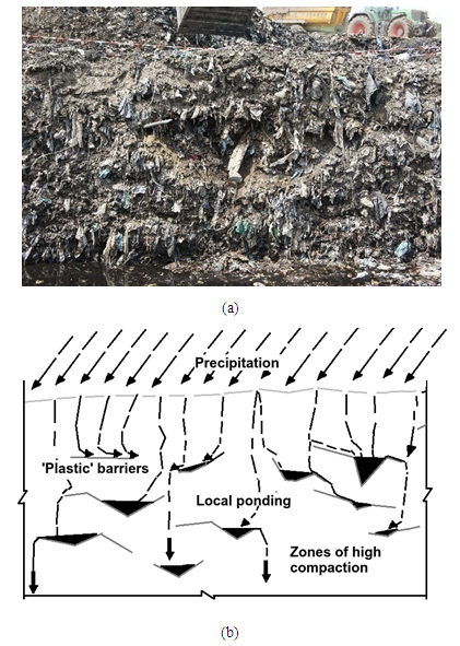Figure 1. Sectional view showing heterogeneous nature of excavated pilot scale landfill located at Landgraaf, Netherlands (a) and simplified overview of flow inside a landfill (figure from Baviskar and Heimovaara (2011) (b))

In this research, we explore the origin of preferential flow in small scale porous systems using a two dimensional (2D) coupled flow and transport deterministic model. In this numerical model, flow is represented by Richards’ equation (RE) (Celia et al., 1990) and transport by advection dispersion equation (ADE) (Bear, 1988; Fetter, 1993). This flow and transport coupled model is formulated in MATLAB (MATLAB, n.d.) as Variably Saturated Flow and Transport (VarSatFT) toolbox. Using VarSatFT, we simulate three different spatially heterogeneous systems and compare their results with a homogeneous one. We consider different types of soils with known van Genuchten properties (van Genuchten, 1980), located systematically in domains of small scale porous systems. These domains are applied with water infiltration in continuous and intermittent patterns of varying rates. The hypothesis is that heterogeneity, in-filtration patterns and infiltration rates act as factors responsible for the origin of preferential flow and non-equilibrium in transport.

The theory for flow and transport in porous media is given section 2. Section 3 contains model description, material parameters and describes different conditions applied on small scale systems. Section 4 reports and explains the effect of material heterogeneity, infiltration patterns and rates in small scale systems. This section also explains controlling factors affecting emission potential, feasibility of single continuum modelling method and suitable models for full scale landfill. Section 5 contains concluding remarks.

2. Theory

2.1. Water Flow

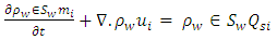
The mass balance equation of fluid flow through porous media can be written as in equation (1) (Pinder and Celia, 2006).

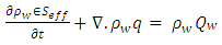(1)

Where,

(2)

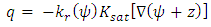
In which is the density of the fluid [M/L³], is the porosity of the medium [L³/L³], is the effective saturation of the medium, q is the Darcy velocity [M/L], is the flow source/sink term [L³/L³T], t is the time [T], is the pressure head [L]. k_r is relative hydraulic permeability function and is the saturated hydraulic conductivity tensor [L/T], for 2D written as where x is horizontal direction and z in the vertical dimension assumed negatively downwards ((by assigning z = 0 at top boundary). An unsteady flow of water in incompressible variably saturated porous medium with no source or sink term can be derived from equation (1) and represented with the mixed-form of RE with Picard iteration process (Celia et al., 1990) as

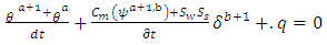(3)

With

(4)

Equation (4) shows the Picard iteration process with a as the time level and b as the iteration stage and dt as time step. C_m is the is differential water capacity [1/L] in which is the water content as a function of S_w is the water saturation, expressed as Ss is the specific storage, which can be presented as , in which, g is acceleration due to gravity [L/T²], is compressibility of water [LT²=M], is coeffiicient of consolidation [LT²/M] and is porosity of the medium [L³/L³].

The van Genuchten equation (van Genuchten, 1980) for the effective saturation , which is needed to solve RE is

(5)

Where

(6)

Where is residual water content [L³/L³], is saturated water content [L³/L³], is effective saturation [no dimensions], is air entry value [1/L], n and m = 1-1/n are van Genuchten parameters for unsaturated flow. van Genuchten’s equation (equation (5)) was used to obtain the relative permeability using Mualems model (Mualem, 1976). Surface ponding can occur when the infiltration is more than infiltration capacity i.e. . The ponding can be approximated using infiltration formula (Green and Ampt, 1911) of surface water balance as shown in equation (7).

(7)

Where is the ponding head at the infiltrating surface, is the infiltration inflow rate occurring at the surface and . is the infiltration capacity of the infiltrating surface. During ponding conditions, the top Neumann boundary is switched into Dirichlet boundary condition with on S1, by solving equation (7).

2.2. Solute Transport

The mass balance of solute transport through a porous medium can be written as equation (8) (Bear, 1988; Fetter, 1993)

(8)

Where

(9)

In which Q_s is the solute source/sink term [L³/L³T], subscript i is the number of species, m is the mass fraction [M/M], t is the time [T], u is concentration flux, q is the advective velocity [L=T], D is hydrodynamic dispersion tensor coefficient [L²/T], for 2D can be written as .

The matrix elements of D can be obtained using equation (10) (Pinder and Celia, 2006) as

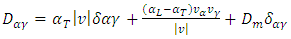(10)

Where,

(11)

where is the dispersion coefficient in respective directions, D_m is the molecular diffusion [L²/T], v is the linear pore water velocity [L/T]. and are the longitudinal and transverse dispersivities [L], respectively. The subscripts and represent the x and z coordinate directions. Substitution of x and z for and yields four values for the dispersion tensor. is the Dirac delta function.

The approach for describing solute transport of a non sorbing, single component through a porous media with no source or sink term can be written as the ADE shown in equation (12).

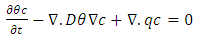(12)

where and is concentration [M/L³].

On further simplification we get equation (13).

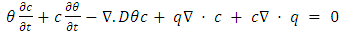(13)

As we have coupled the transport equation with the flow equation,

Thus, we can write equation (13) as equation (14).

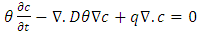(14)

where q and are variables coupling the transport equation with the water flow equation, mathematically presented in equation (2) and equation (6).

The initial condition for the ADE can be expressed as

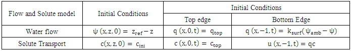
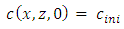(15)

where is initial concentration [M/L³].

The boundary conditions can be expressed as a Dirichlet boundary condition on S1 (See equation 16) and a Robbins boundary condition on S2 (See equation 17). Where S1 + S2 = S is the total boundary region.

(16)

(17)

where is concentration at the boundary condition [M/L³].

In the Eulerian-Lagrangian method, the Eulerian and Lagrangian time derivatives of concentration are related to each other through an advective transport term (See equation (18)) (Ewing and Wang, 2001).

(18)

The Lagrangian time derivative can be equated to the dispersion term as shown in equation (14). The dispersion term is solved on Euler grid. Whereas the advective term from the right hand side of equation (18) is solved by Lagrangian method (MIC method).

In Lagrangian method, the concentration c, and the x and z components of linear velocities v are initially distributed on the dimensionless markers (Refer equation (11) for v) (Gerya and Yuen, 2003). These Lagrangian markers are advected using equation (19).

(19)

where and are the location of the markers in x and z direction at time t, and and are the location of the markers in x and z direction at time The and are the linear velocities of the markers. The change in distribution of the markers due to advection is utilized for interpolating the concentration from the markers to the surrounding nodes. This interpolation of concentration from nodes to markers and vise-verse is carried out at every time step.

3. Materials and Methods

3.1. VarSatFT Simulator

The water flow was modelled using mixed-form of RE. The non-linearity of RE was solved using Picard iteration process (Celia et al., 1990). The ADE for solute transport consisted of a non-sorbing single component species, which was solved using Eulerian - Lagrangian approach. In this approach the dispersion was solved on Euler nodes and the advection was solved on Lagrangian markers using modified marker-in-cell method (MIC) inspired by Gerya’s (Gerya and Yuen, 2003) MIC method (Baviskar, 2016). The discretized form of flow and transport equations were implemented using finite difference method in VarSatFT toolbox, formulated in MATLAB. The VarSatFT simulator has been verified by simulating variety of o flow and transport problems described in Baviskar (2016).

3.2. Description of Small Scale Systems

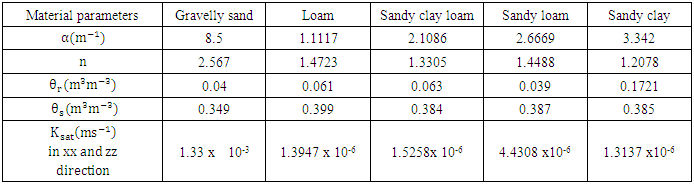
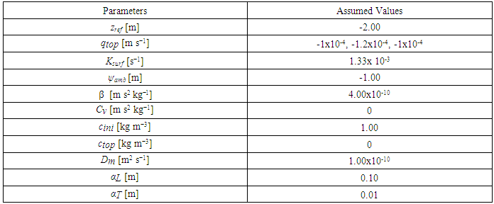
In this section we describe the spatial scenarios, the boundary conditions and the simulation procedure applied on the small scale systems. These small scale systems were build of domain size 1:0 m 1:0 m dimensions. The domains were discretized into elements of size 0:05 m.

We have considered different spatial scenarios in small scale systems. We have named them as Gravelly sand and Plastic (GP); Gravelly sand Loam and Plastic (GLP); Five Materials (FM) (See Table 1). Their simulation results were compared with a Homogeneous (H) scenario domain system. Detailed diagrams of these different spatial scenarios are shown in figure 2. The material properties considered for different soil profiles are indicated in Table 2. These properties were referred from Schafer (2001) and Thoma et al. (2013).

Table 1. Abbreviations for different spatial and infiltration scenarios

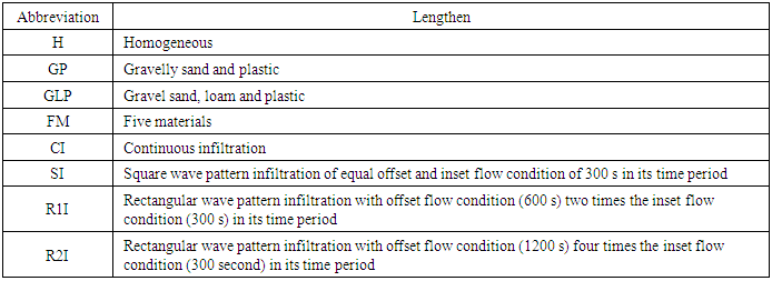
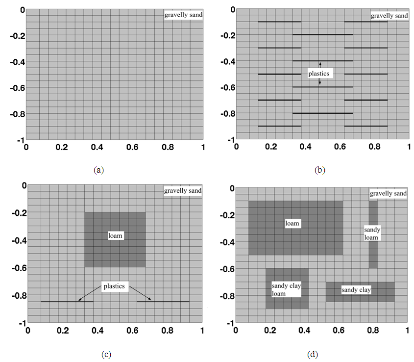Figure 2. Spatial scenarios: H (a); GP (b); GLP (c) and FM (d)

The initial and boundary conditions applied on the small scale systems for flow and transport related to our study is listed in Table 3. For water flow, the initial condition was a highly unsaturated. The Neumann boundary condition was implemented at the top edge, where q_top is infiltration applied with different rates in continuous (CI), square wave (SI) and rectangular wave patterns (R1I and R2I) (See figure 3 (a) and Table 1). The infiltration in rectangular wave pattern was of two types with different no-flow pulse width for its time period. The Robbins boundary condition was applied at the bottom edge, where is the surface permeability and is the ambient pressure head. For impermeable plastics in some of the spatial scenarios, we assume that K = 0 m s^-1 at the required inter-nodes.

Table 2. Material properties for soil profiles used in different small scale systems were considered from Schafer (2001) and Thoma et al. (2013)

Table 3. Initial and Boundary conditions used in simulations

For solute transport, the initial concentration was considered to be uniformly distributed throughout the domain of system. A Dirichlet boundary condition was applied to the top edge, and a Robbins boundary condition of zero concentration gradient was applied at the bottom edge. The left and right edges were defined to be impermeable for the flow and transport. The values for the initial, boundary conditions and other parameters are listed in Table 4.

Table 4. Assumed parameters used in simulations

In this study, we generated results for 48 different scenarios (4 spatial scenarios; each spatial scenario applied with 4 different types of infiltration patterns; each pattern has 3 different types of infiltration rates). The cumulative of infiltrations are shown in figure 3(b). All these systems were simulated for a time range of 5 days with the temporal discretization of 100 s. The implications of heterogeneities, infiltration rates and patterns on spatial distributions of flow and transport are investigated through these small scale systems.

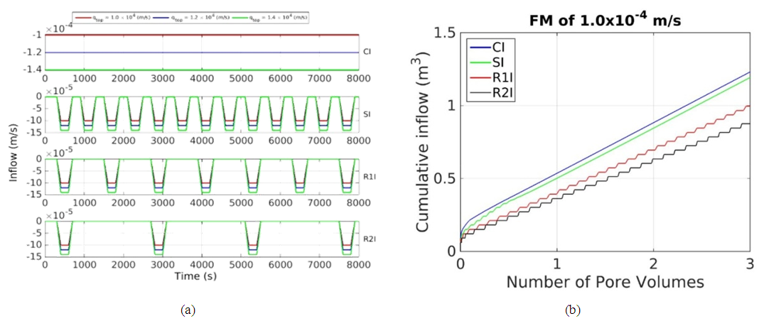Figure 3. Infiltration scenarios: Infiltration patterns and rates applied (a). Cumulative of infiltrations for 1:0 10 4m s 1 rate of all infiltration patterns (b)

4. Results and Discussion

In this section we analyses how heterogeneity and infiltration patterns and rates affect the flow and transport in small scale systems. We only consider a few of the spatial scenarios and generic boundary conditions as described in section 3.2.

4.1. Distributions of Flow and Transport Observed in Spatial Distributions

The results of spatial distribution of the pressure head, water content and solute concentration are illustrated in this section. The flow and transport in the homogeneous system (H) are only in vertically downward directions. Flow and transport in the gravel-plastic system (GP) flow along longer flow paths following the orientation of the plastics. In the other systems with a mixture of more materials (GLP and FM), the presence of plastics and soils with low and high permeabilities cause horizontal flow along the plastics and low permeable fine soil materials. In addition the solute will only slowly leach from the fine soil materials with lower permeabilities due to a significantly reduce advective transport component. This contributes to a lower rate of decrease in solute concentration levels (Das et al., 2004).

We show simulation results for all spatial scenarios (FM, GPL, GP and H) with a infiltration rate of 1:00 10⁴ m s ¹ and a pattern R2I. They were observed at the end of 12 h of total simulation time where 0:54 m³ was the cumulative amount of water infiltrated.

The results for the H spatial scenario are shown in figure 4. The pressure head contours are horizontal and have decreasing values along the depth of domain. This indicates that the flow is only due to vertical pressure gradients (figure 4(a), (b), (c)). The solute concentrations are completely flushed at 2.95 pore volumes at the observed time (figure 4(c)).

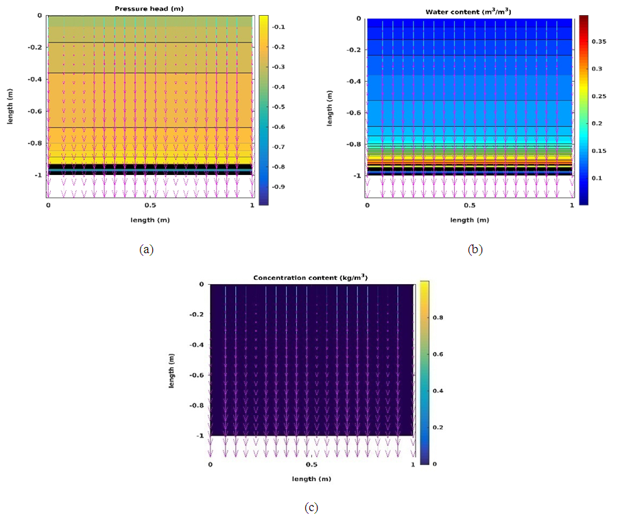Figure 4. Distribution of pressure head (a) water content (b) and solute concentration for the H spatial scenario subjected to an infiltration rate of -1.00 x10-4 m s-1 with the R2I inflow pattern. Results are shown after 12 h of the total simulation time

In figure 5 the results for the GP spatial scenario show a significant variation in pressure head and water contents near the plastic layers. Increased water con-tent above, and lower values below (figure 5(a), (b)). Vertical flow is inhibited at the position of the plastic leading to the development of perched water table. These local perched water tables induce horizontal pressure gradients causing horizontal flow along the periphery of plastics (figure 5(a), (b), (c)). Three main types of streamlines can be discerned in the GP scenario. The first is in the middle of the model domain and are the longest streamlines flowing along the plastic sheets in an oscillatory fashion. The second can be found near the left and right edges of the domain and are the shortest in length as they are not influenced by the presence of the plastic. Finally the third type are streamlines which fall between these two extremes. The figure with solute concentrations clearly indicates the shadow effect caused by the diversion of water by the presence of plastics (figure 5(c)). Even after flushing 2.36 number of pore volumes some salt remains present at the bottom of the domain.

Figure 5. Distribution of pressure head (a) water content (b) and solute concentration for the GP spatial scenario subjected to an infiltration rate of 1.00 x 10-4 m s-1 with the R2I inflow pattern. Results are shown after 12 h of the total simulation time

The contours and streamlines in the GLP scenario shown in figure 6 illustrated the presence of perched water tables on top of the fine loam block and plastics caused by the lower hydraulic conductivities compared to the back-ground gravelly sand material (figure 6(a), (b)). The perched water tables induce horizontal pressure gradients in time causing flow directed along the periphery of the loam block and plastics (figure 6(a), (b), (c)). The low saturation of the gravelly sand below the loam block, leads to lower relative permeabilities. Capillary suction retains the water in the block of loam (figure 6(b)). No advective solute transport can take place in the block of loam, only diffusion can occur, driven by the gradients in concentration near the edges of the block of loam (figure 6(c)). Clearly extreme differences in material properties cause an incomplete flushing of the solute concentrations from the loam block at the observed time even though 2.19 pore volumes have been flushed.

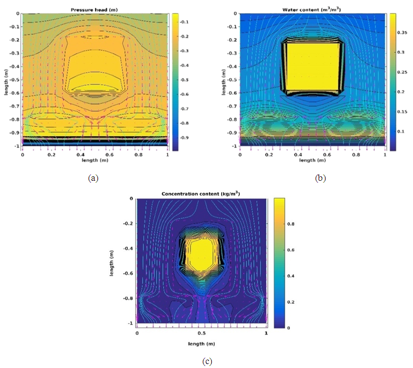Figure 6. Distribution of pressure head (a) water content (b) and solute concentration (c) for the GLP spatial scenario subjected to an infiltration rate of -1.00 x 10 -4 m s-1 with the R2I inflow pattern. Results are shown after 12 h of the total simulation time

The results of the FM-scenario show a combination of the effects found in the previous scenarios (See figure 7). Perched water tables develop on top of the fine soil blocks (loam, sandy clay loam, sandy loam, sandy clay) because of the difference in hydraulic conductivity (figure 7(a), (b)). The perched water tables induce horizontal pressure gradients which vary in time. As a result flow is directed along the periphery of these fine material blocks (figure 7(a), (b), (c)). Due to the reduced advective transport in these fine material blocks, solutes are retained because diffusion is a slow process (figure 7(c)). Thus solute concentrations are retained in the domain at 1.73 flushed pore volumes at the observed time.

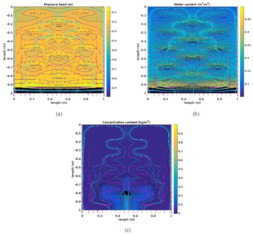
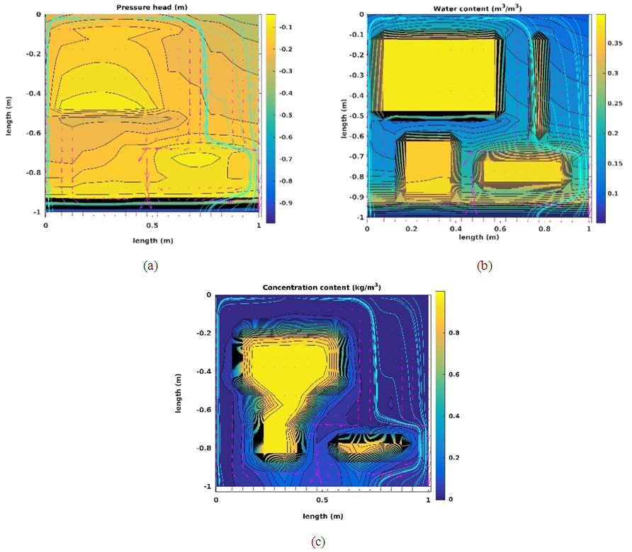Figure 7. Distribution of pressure head (a) water content (b) and solute concentration (c) for the FM spatial scenario subjected to an infiltration rate of -1.00 x 10-4 m s-1 with the R2I inflow pattern. Results are shown after 12 h of the total simulation time

The results observed in figures 4, 5, 6 and 7 clearly show that the presence of plastics and fine soil blocks leads to emergence of horizontal flow. The anisotropic nature of permeabilities in heterogeneous scenarios lead for a development of horizontal pressure gradients. More horizontal pressure gradients are observed for the scenario with higher heterogeneities (FM>GLP>GP). Retention time of solutes depends on the length of the stream lines which tends to increase when the heterogeneity in the domain increases. Presence of impermeable layers also leads to a focusing of streamlines with depth in unsaturated systems. This focusing causes shadow zones below impermeable layers which will retain solutes as they are not flushed. Materials with low hydraulic conductivity values can retain solutes for a long time as the only leaching process is diffusion. The larger the size of such blocks of materials, the longer solutes will be retained. This leads to formation of the immobile and mobile regions, where immobile regions retain solutes much longer than mobile regions. Therefore in-creased heterogeneity leads to an increased variation in lengths of streamlines and therefore an increased variation in travel times for water moving through the domain. At the macroscopic level, the lowest travel times can be considered to be flowing through preferential flow paths (Kohler et al., 2001; Šimunek et al., 2003; Šimunek and van Genuchten, 2008). However, one should realize that there can be a very wide distribution of travel times. In principle two dominant mechanisms can be identified: 1) increased travel time due to increased streamlines and 2) long retention of salts due to presence of materials with low hydraulic conductivity.

4.2. Average Total Drainage Relationships

The simulation results allow us to calculate total drainage relationships for the complete model domain for the different scenarios. Here we show the normalized average solute concentrations and average solute masses obtained in the discharged leachate as a function of the number of flushed pore volumes.

4.2.1. Effect of Heterogeneity on Flow and Transport

The results shown in figure 8 illustrated the impact heterogeneities have on the leachate. The solute breakthrough for scenarios GP, GLP and FM reflect the intermittent infiltration pattern R2I. The variation in solute concentration in the breakthrough curves (BTCs) is caused by the timing between flow and no-flow during the simulation. Solute concentrations only increase only in the heterogeneous scenarios (in order of FM>GCP>GP) and not for homogeneous (H) scenario. The increase is caused by local diffusion of solute from the relative immobile pore water to the mobile pore water during stagnant flow conditions. When flow starts again, the solute leaches with the mobile water.

In addition we also observe an early breakthrough of solute for the different heterogeneous scenarios (in order of FM followed by GP and then by GLP). The breakthrough for scenario H is obtained at 1 pore volume. Relatively longer streamlines causes a broader break through curve for scenario GP as compared to other heterogeneous scenarios and homogeneous scenario. Scenarios GLP and FM requires more than 1 pore volume for complete drainage of solute because slow diffusion from the immobile to mobile pore water. The tailing of solute for scenario FM is longest as compared to that observed in GCP, GP and H.

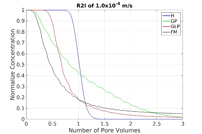Figure 8. Effect of Heterogeneity: normalized average solute concentration against number of pore volumes obtained for all scenarios applied with R2I infiltration pattern with -1.0 x 10-4 m s-1 infiltration rate

The difference in pore volumes required to drained the solute can be partly be explained by the differences in porosity distributions (Lunati et al., 2003).

The porosity in heterogeneous scenarios is in order of FM>GLP>GP. However, more important is the fact that differences in hydraulic conductivity prevent water from flowing through a significant part of the domain. Diffusion instead of advection leads to the long tailing and therefore, the large number of pore volumes required to leach the solute.

4.2.2. Effect of Infiltration Pattern on Flow and Transport

Figure 9 shows the effect of varying the infiltration patterns where we move from continuous infiltration to more and more heterogeneous infiltration (CI, SI, R1I, and R2I). For the H-scenario, it appears that solute breakthrough occurs earlier with the CI and SI infiltration patterns compared to those observed with the R1I and R2I infiltration patterns. The difference between these scenarios is that the variation in water content throughout time is larger for the R2I and R1I scenarios because the water drains in the conditions with no flow. This result is physically not realistic as it should disappear when expressing the leached solute as a function of pore volume. Therefore, this result indicates an error in the implementation of the model. The linearization during finite discretization in time leads to this error.

For the GP-scenario, solute tailing is significantly longer for the R2I infiltration pattern than observed for R1I, SI and CI. The breakthrough curve breaks in four parts (See figure 9(b)), the first three parts indicates the three types of streamlines classified with respect to their lengths and the last part indicates the diffusion process. For the GLP-scenario, all results for infiltration patterns (CI, SI and R1I) are similar, only infiltration pattern R2I differs. For the FM-scenario, a longer tailing is observed for the R2I pattern compared to R1I, SI and CI.

The continuous infiltration for the CI-pattern leads to a steady state water content in the domain. The time of the no-flow conditions in the SI-pattern is apparently so-small that no significant drainage could occur. In a dry column, water can be stored in the pore-space before drainage occurs, the temporal variation in storage is largest in scenario R2I. In a heterogeneous porous system where concentration gradients are present, increased storage during infiltration will lead to relatively more time for solute exchange to take place before water is discharged from the system as leachate. This will cause larger variations in leachate concentration. The slow exchange implies a non-equilibrium between the solute concentrations in the immobile and mobile pore water.

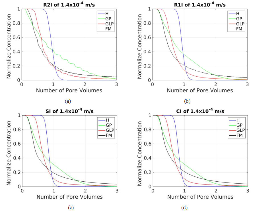Figure 9. Effect of Infiltration pattern: Normalize average solute concentrations plot-ted against number of pore volumes obtained from drainage for all spatial scenarios (H, GP, GLP and FM) applied with different types of infiltration patterns (R2I, R1I, SI and CI) with -1.4 x 10-4 m s-1 infiltration rate

4.2.3. Effect of Infiltration Rates on Flow and Transport

Figure 10 shows breakthrough curves for the FM-scenario with the R2I in-filtration pattern subjected to all three infiltration rates -1.0 x 10^-4 m s^-1 , -1.2 x 10^-4 m s^-1 and 1.4 x 10 ^-4 m s^-1. The enlarged plots show details of the early drainage and long tailing for the three different infiltration rates. It is clear that slow diffusion from the immobile water leads to a rise in concentration of the mobile water. The differences between the three infiltration rates is caused by a larger dilution in the mobile water for the highest flow rate, the residence time of the mobile water during flushing is shorter. As a consequence, the mobile water flushes faster in the high flow rated condition. However, the large volume of immobile water dominates the tailing. Presence of non-equilibrium exchange in a system with variation in infiltration regime has a significant impact on the dynamics in the leachate concentrations. Decreasing amounts of mobile pore water lead to larger variations in leachate concentrations.

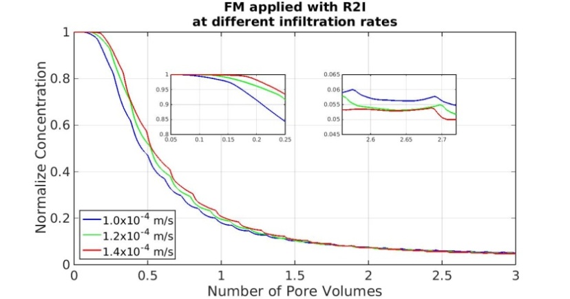Figure 10. Effect of Infiltration rates: normalized average solute concentration against number of pore volumes obtained for FM scenario applied with R2I infiltration pattern with -1.0 x 10-4 m s-1, -1.2 x 10-4 m s-1 and -1.4 10-4 m s-1 infiltration rates

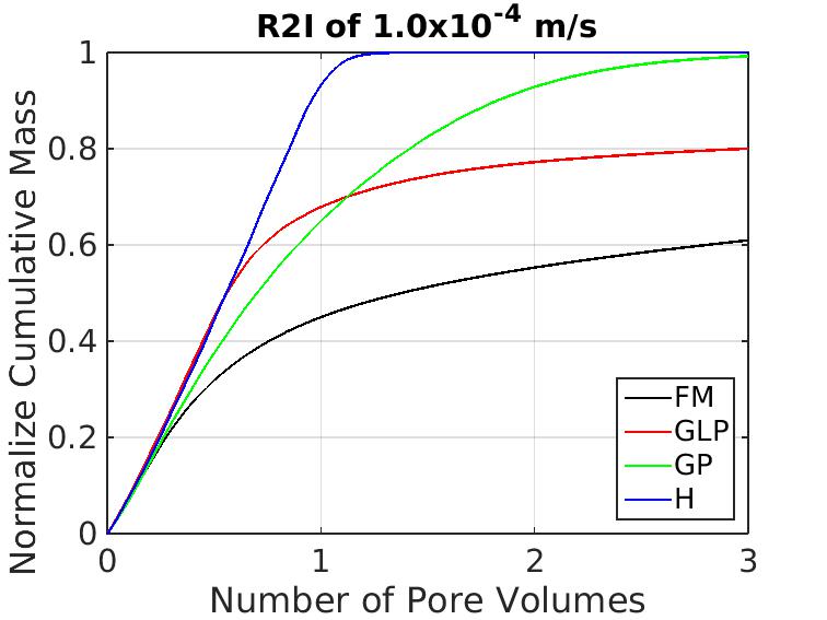
4.2.4. Factors Controlling Emission Potential

The normalized cumulative mass in the leachate as a function of flushed pore volumes is shown in figure 11. The outflow mass is normalized to the initial amount of solute present in the model domain. As expected, complete flushing occurs for the H-scenario after about 1 pore volume. The variation in travel times in the GP-scenario and the development of shadow zones requires significantly more water to be infiltrated to achieve complete flushing. The presence of zones with low hydraulic conductivity in the GLP and FM scenarios prevent complete flushing. The mobile zone flush quickly, slow diffusion causes a long tailing.

Bun et al. (2013) proposed that the solute mass in the waste body at a certain point time should be considered to be the emission potential of a full scale landfill. The simulations on small scale systems discussed in this section 4.2.2 and 4.2.3 show that high rates with the CI-pattern removes solute most effectively because of maintaining the largest gradients in concentration between the mobile and immobile water. In full scale landfills where rainfall is in general intermittent, it takes more than 10 years to obtain a drainage of 1 pore volume. Increasing infiltration in a relatively continuous mode in order to increase the cumulative amount of water infiltrating would increase the reduction of emission potential of a landfill. However the tailing effect is difficult to address. After flushing the mobile pore volume, concentrations in the leachate are dominated by the ratio between the mobile and immobile pore volumes.

Figure 11. Normalize cumulative average solute mass against number of pore volumes obtained from drainage for all scenarios for R2I infiltration pattern of -1.00 x 10-4 m s-1 rate

In full scale landfills, the volume of preferential pathways responsible for draining 95% of the infiltrating water can be only 0.2% of the total volume (Fellner and Brunner, 2010) and leachate concentrations are highly correlated with discharge rate.

4.3. Feasibility of Single Continuum Modelling Method for MSW Landfill

Richards’ equation has often been used for modelling the production of leachate from landfills (Gholamifard et al., 2008; McDougall, 2007). This common modelling approach is based on assumptions of homogeneity of the landfill media (Ahmed et al., 1992; Demetracopoulus et al., 1986; Vincent et al., 1991). In full scale landfill the heterogeneity scale may vary from the size of a gravel to a large plastic sheet and may change in time. In this paper we show that preferential flow exists even for a smallscale heterogeneous systems (See figure 8). So it is very likely that preferential flow occurs within the representative elementary volume (REV) of 1 cubic meter, used in continuum models by McDougall (2007) and Gholamifard et al. (2008). As a consequence the results obtained using such single continuum models for a full scale landfill do not match field observations (Rosqvist et al., 2005; Rosqvist and Destouni, 2000; Ugoccioni and Zeiss, 1997). Preferential flow in MSW landfill occurs only through 0.2-10% of the volume of landfill (Fellner et al., 2009; Ugoccioni and Zeiss, 1997).

In addition, in closed landfills the location of the different waste materials is not known. There is a large variation in the material properties of waste and therefore varying chemical composition (El-Fadel et al., 1997; Ziyang et al., 2009). Material properties of waste inside landfill cannot be quantified. Therefore the single continuum deterministic modelling approach for full scale landfill becomes unrealistic (Bun et al., 2013).

4.4. Suitable Modelling Methods for MSW Landfill

In modern landfills, the easily available parameters obtained during landfill monitoring are the infiltration rate (i.e rainfall or irrigation inflow rate), the outflow discharge and the electrical conductivity of the leachate obtained from the drainage layer (W. van Vossen and Heyer, 2009; W. J. van Vossen and Heyer, 2009). Jury (1982); Jury and Roth (1990); Jury and Stolzy (1982) has shown how these types of inlet and out-let parameters could be related together and utilized as an modelling approach for flow and transport in the vadose soil zone. Similarly Zacharof and Butler (2004a, 2004b) relates these input output parameters to model landfill leachate quality and quality. Therefore, it seems that models which take the preferential flow and non-equilibrium in transport into account is better than the single continuum - based models.

The drainage relations obtained in section (4.2.1) can be described using non-equilibrium models. For instance the drainage relationships for GLP and FM scenarios can be modelled using a dual or a multi-permeability model (Bendz et al., 1998; Šimunek et al., 2003). In the GP scenario, the non-equilibrium emerges due to varying length of streamlines so we could use a stream tube model to model this behavior (Matanga, 1996).

In figure 12 we plot outflow mass and discharge along number of pore volumes for FM scenario for R2I infiltration with 1.0 10⁴ m s^-1 rate. For same number of pore volumes, an increase in outlet solute mass corresponds to an increase in discharge rate (See, the BTC of solute mass and discharge, along same vertical grid lines). This is observed until all the mass is drained out from the domain. The negative sign for the solute mass suggests draining in downward direction. Using this relation the type and rate of infiltration can be designed to optimize the required emission potential of a landfill. However, this type of correlation between the solute concentrations or EC measurements and the discharge outflow is observed only for intermittent patterns of infiltration or for rainfall precipitations. This relationship can be used to determine the probability distribution of the solute transport time. The transfer function approach by Jury and Roth (1990) can be utilized to determine the emission potential of full scale landfill.

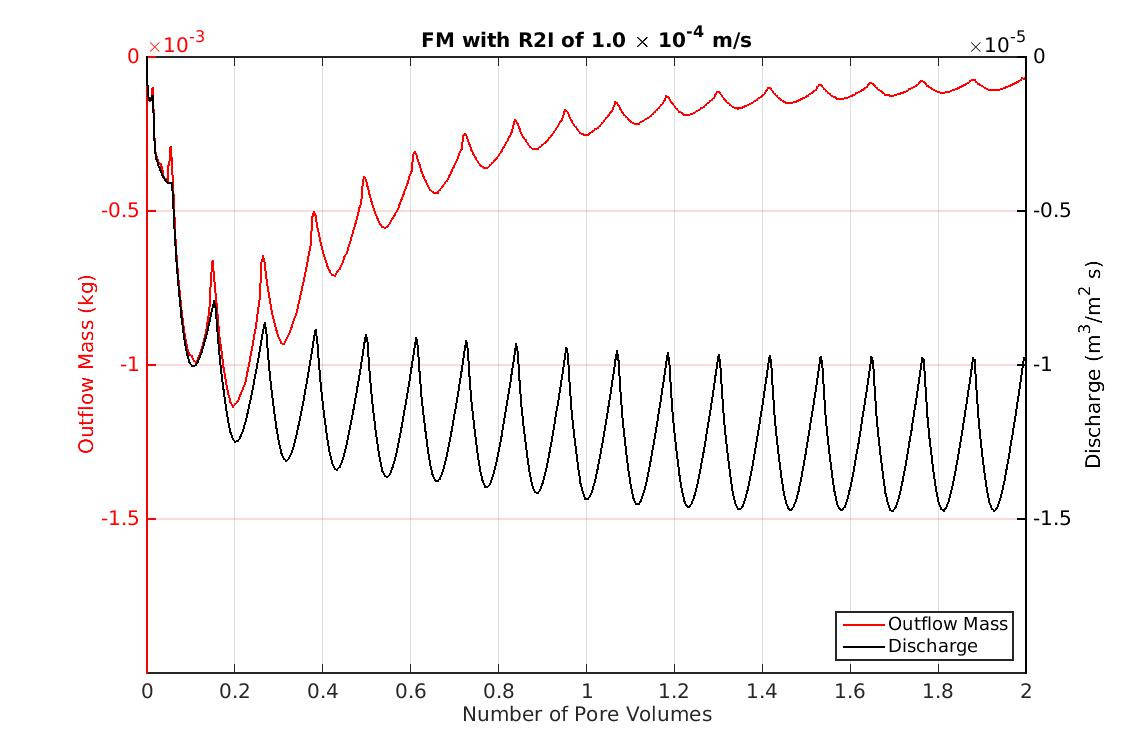Figure 12. Outlet solute mass along against number of pore volumes obtained at drainage for heterogeneous scenario FM for -1.0 x 10 -4 m s-1 rate and R2I pattern

5. Conclusions

In this research, we show that introducing spatial heterogeneities in small scale systems can lead to preferential pathways and, therefore, emergence of non-equilibrium behavior in solute transport. It is highly probable that the spatial distribution of pressure head, water content and solute concentration observed in this study is similar to locations present in existing landfills. The heterogeneous scenarios show an increase in travel time distributions along a range of streamlines compared to travel time distributions in homogeneous scenarios. This is a strong indication of the emergence of preferential flow in heterogeneous scenarios. The emergence of solute non-equilibrium effects is due to the emergence of concentration gradients in heterogeneous systems due to local variations in water content and solute transport.

The averaged total drainage results show that larger numbers of pore volumes are required to flush solute mass from heterogeneous porous media. More efficient flushing is achieved when continuous modes of infiltration are used. Decreasing infiltration rates slightly increases the non-equilibrium in transport, reducing efficiency of flushing. For flow and transport in heterogeneous small scale systems, infiltration rate and infiltration pattern acts as the controlling factors for non-equilibrium in transport due the induced variations in water content in the system.

Reducing the emission potential from a full scale MSW landfill with continuous infiltration requires large amounts of water, hence it is infeasible. Especially when taking the heterogeneity of a landfill in to account. Slow diffusion from the immobile pore water will require a very long time. Actively approaches aiming to reduce residence time of water in the waste body are probably the most effective approach for controlling emissions via leachate.

The single continuum equilibrium coupled flow and transport model we developed shows the emergence of non-equilibrium effect in small scale heterogeneous systems. These results provide compelling evidence that preferential flow for a full scale landfills is most likely. However, using a single continuum deterministic modelling methods based on volume averages or empirical values of these waste properties gives different results from field observations is impractical because of the very small REV scale required. Upscaled approaches which consider the non-equilibrium transport provide better results corresponding to field observations. We recommend utilization of transfer function approach to model leachate dynamics of full scale landfills.

ACKNOWLEDGEMENTS

The authors would like to thank Erasmus Mundus Lot-13 scholarship and Delft University of Technology for organizing the funds for this research. The authors declare no conflict of interest.