-
Paper Information
- Previous Paper
- Paper Submission
-
Journal Information
- About This Journal
- Editorial Board
- Current Issue
- Archive
- Author Guidelines
- Contact Us
American Journal of Environmental Engineering
p-ISSN: 2166-4633 e-ISSN: 2166-465X
2018; 8(5): 181-200
doi:10.5923/j.ajee.20180805.03

Can Prior Experience Provide a Means to Predict Success of Future Aquifer Storage and Recovery Systems?
 Abstract
 Reference
 Full-Text PDF
 Full-text HTML
Frederick Bloetscher
Florida Atlantic University, Boca Raton, FL, USA
Correspondence to: Frederick Bloetscher, Florida Atlantic University, Boca Raton, FL, USA.
| Email: |  |
Copyright © 2018 The Author(s). Published by Scientific & Academic Publishing.
This work is licensed under the Creative Commons Attribution International License (CC BY).
http://creativecommons.org/licenses/by/4.0/

This paper is the result of analysis data gathered from a 2013 survey of all 204 Aquifer Storage and Recovery (ASR) sites in the United States. That 2013 ASR site survey included all active, inactive, test and study sites, and collected both operational and construction details. The differences between the operational and inactive sites are of particular interest because the differences are where the most information can often be gleaned as to the potential for success of the test and study sites. The statistical analysis utilized in this analysis focused on the active and inactive sites – all sites in study mode and early stages of development were not included in the initial analysis. The intent was to determine is a predictive model for ASR success could be developed for the test and study ASR sites, as well as potential future sites. The results improve on prior papers by the author related to ASR system success and provides insight on what factors improve the likelihood of successful ASR projects. Using the results of the PCA, a linear regression model was developed for the active and inactive sites, and applied to the test and study sites to predict their likelihood of success. The results provide insight into the potential for success in the 50+ test/study sites that may be years for full development.
Keywords: Groundwater Storage, Recharge, Predicting Success
Cite this paper: Frederick Bloetscher, Can Prior Experience Provide a Means to Predict Success of Future Aquifer Storage and Recovery Systems?, American Journal of Environmental Engineering, Vol. 8 No. 5, 2018, pp. 181-200. doi: 10.5923/j.ajee.20180805.03.
Article Outline
1. Introduction
- Water supply challenges exist throughout the world. As a result, in drought or water limited areas, the ability to store water for later use has value for sustainability of the local community. AWWA Manual M21 [1] divides aquifer storage programs into four categories: Artificial Aquifer Creation, Aquifer Recharge, Aquifer Reclamation, and Aquifer Storage and Recovery (ASR). All of these approaches are used as part of the water supply industry to ensure that sustainable water resources are available for agricultural, environmental and urban uses. This paper focusses on the ASR portions only and utilizes the dataset developed in conjunction with AWWA Manual M-63 [2-4]. ASR is touted as a viable concept in the management of both potable and non-potable water supplies. Utilities pursue ASR programs to increase the efficiency of system operations to utilized unused water treatment plant capacity to treat water and pump it into an aquifer for later withdrawal for augmentation of water supplies at a later point of time to avoid the need to construct plants only for peak demands [2-4]. The injection applications include potable water, raw surface and groundwater, and reclaimed wastewater. The storage period can be over multiple months to allow the stored water to meet the next high demand season, an emergency such as a severe drought or during an interruption of water withdrawal due to equipment breakdown.The concept of ASR has only been applied in the United States since the late 1960s and little development occurred until the 1990s (see Figure 1). As a result, until recently, the number of sites has been limited, and the fact that it may take 10 years to develop an operational ASR system, means that truly acquiring data has only recently become available to a number of sites. Hence, the first complete survey of ASR sites was completed in 2013, and little has changed since that time [3, 4]. Dataset was the first comprehensive analysis of the 204 sites in the US. U.S. EPA and environmental agencies in each state with ASR wells were contacted by phone or email to whether the state had such programs in place or not, and where they might be located. The list of ASR sites identified by the regulatory agencies was a critical component of the project because while prior inventories were prepared by regulatory agencies and consultants, none were complete and most excluded projects that were no longer active [5-9]. In each of these documents, the goal was to provide information on successful ASR sites as case studies and were relatively limited to a few sites as opposed to a nationwide survey (for example, AWWA [5] included only 4 sites in Florida, as opposed to 54). Hence, while AWWA [5] and Bloetscher et al [6] provided more extensive summaries that the texts by other authors, these reports were also very limited in scope. No analysis of the data was conducted to identify trends, success and challenges for ASR projects. The first to analyze the successes and challenges encountered by ASR projects were Bloetscher et al [3, 4].
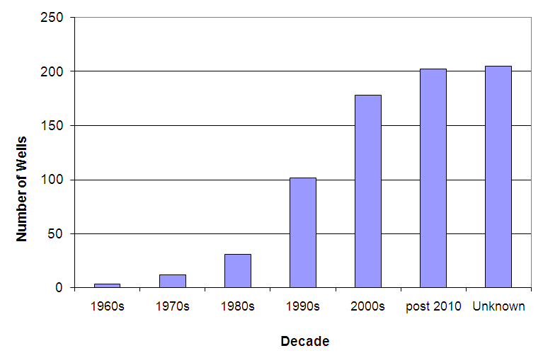 | Figure 1. Cumulative ASR sites by Decade |
2. Methodology
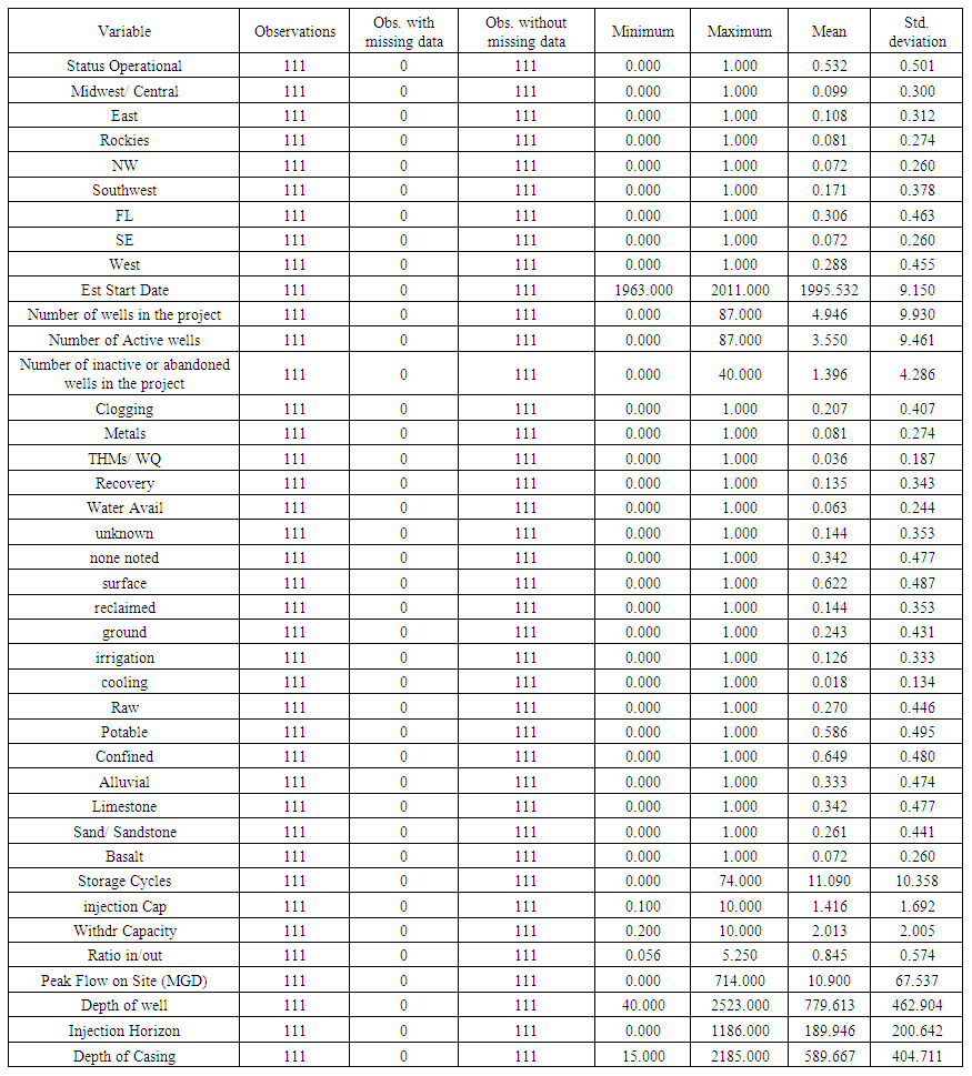
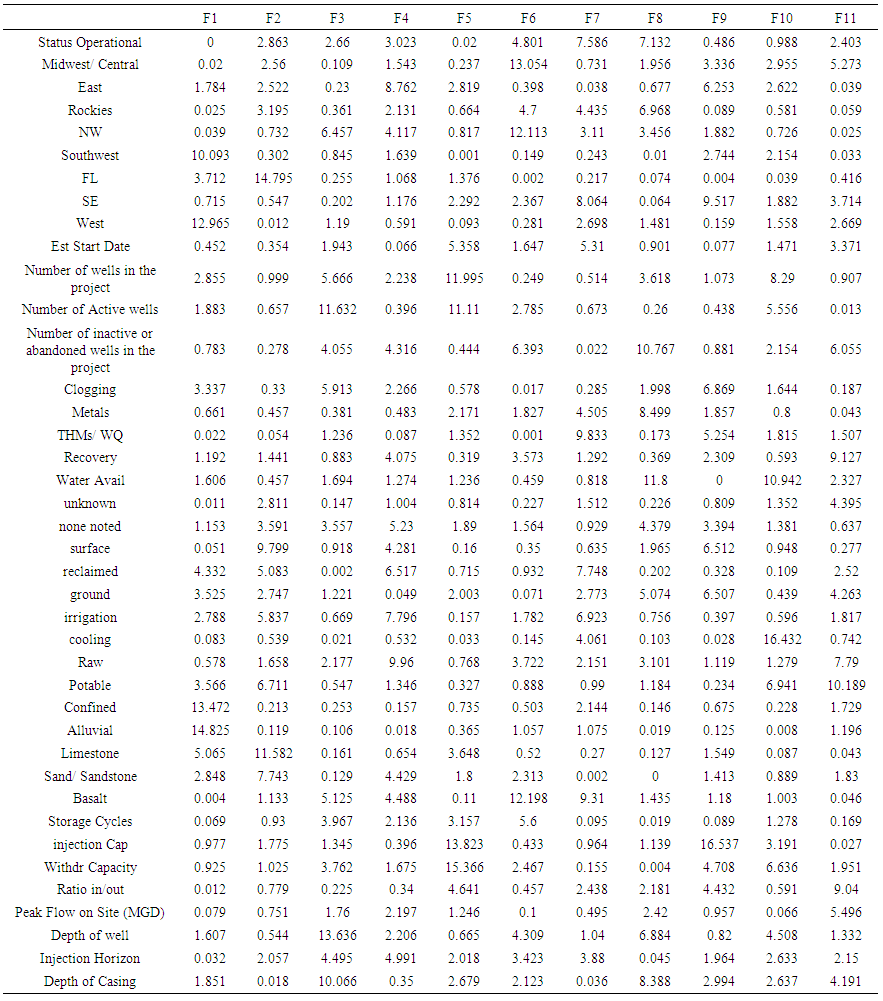
- The data utilized for this analysis are noted in Table 1, which were variables extracted from the 2013 ASR site inventory [2], and then converted to numerical variables as required for the statistical methods employed (see Tables 2 and 3). Also, information was updated to reflect known changes in the ASR wells. Am0ong the issues noted was that complete information was not available for all sites and decisions needed to be made to determine is those ASR sites would be retained or the variables deleted. For example, the salinity of the injection zone is relevant when injecting fresh water into a brackish zone. Freshwater will float based on the principles of differential density, creating a challenge for recovery of the injected water. However, the dataset denoted that the majority of sites were injecting into freshwater (total dissolved solids under 1000 mg/L) except in south Florida [2]. As a result this variable was deleted as opposed to deleting several dozen sites that did not report the salinity. The decisions were important because those sites with incomplete data, or those variables that were incomplete, cannot be used in principal component analysis which would reduce the available data considerably. Likewise, the casing material was commonly not reported and the confined layer material was not well defined. These variables were also deleted to permit as many sites to remain as possible.
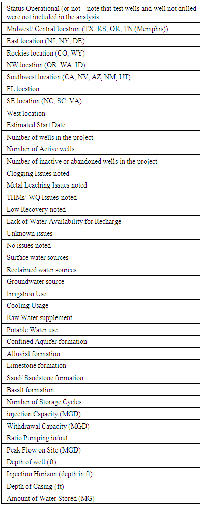 | Table 1. Variables used in ASR Analysis |
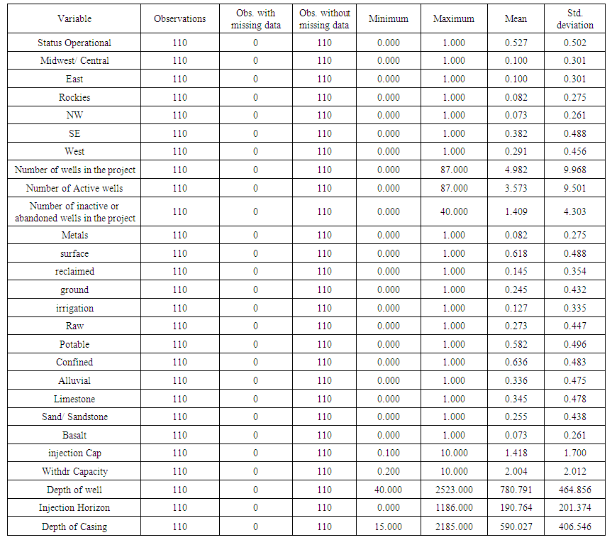
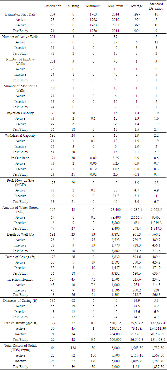 | Table 2. Descriptive statistics of continuous variables related to the ASR sites in the United States |
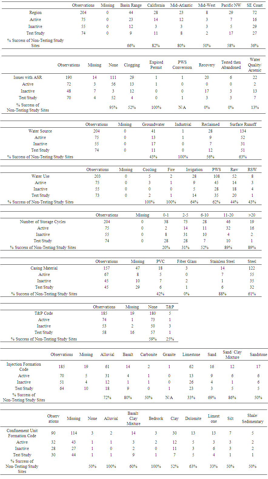 | Table 3. Descriptive statistics of categorical variables per ASR program status in the United States |
2.1. PCA and FA Analysis
- The factor analysis method dates from Spearman [10] and continues to develop. Today, there are two main types of factor analysis: Exploratory factor analysis (or EFA) and Confirmatory factor analysis (or CFA). EFA is used by XLStat® to reveal the possible existence of underlying factors which give an overview of the information contained in a very large number of measured variables. For EFA, the structure linking the variables is initially unknown, but the number of factors is assumed. CFA uses a method identical to EFA but the structure linking underlying factors to measured variables is assumed to be known [11].Principal Component Analysis (PCA) is popular multivariate technical mainly used to reduce the dimensionality of p multi-attributes to two or three dimensions [11-13]. PCA is a special case of factor analysis (where k, the number of factors, equals p, the number of variables). While FA assumes a number of factors, PCA is used to reduce the number of variables to factor sets, while maximizing the unchanged variability in order to obtain independent (non-correlated) factors [14]. The mathematics of PCA uses an orthogonal transformation convert observations of possibly correlated variables into a set of values of linearly uncorrelated variables called principal components [13-16]. PCA uses a multivariate statistical parameter called an eigenvalue, which is a measure of the amount of variation explained by each principal component. PCA summarizes the variation in a correlated multi-attribute to a set of uncorrelated components, each of which is a particular linear combination of the original variables [17]. PCA is the simplest of the true eigenvector-based multivariate analyses. A Scree Plot is a simple line segment plot that shows the fraction of total variance in the data as explained or represented by each component [18].There are several uses for PCA, including [11]:• The study and visualization of the correlations between variables to hopefully be able to limit the number of variables to be measured afterwards;• Obtaining non-correlated factors which are linear combinations of the initial variables so as to use these factors in modeling methods such as linear regression, logistic regression or discriminant analysis.• Visualizing observations in a 2- or 3-dimensional space in order to identify uniform or atypical groups of observations.Two methods are commonly used for determining the number of factors to be used for interpreting the results: the Scree test [19] is based on the decreasing curve of eigenvalues. The number of factors to be kept corresponds to the first turning point found on the curve. However, these representations are only reliable if the sum of the variability percentages associated with the axes of the representation space are sufficiently high. If this percentage is high (for example 80%), the representation can be considered as reliable. If the percentage is reliable, it is recommended to produce representations on several axis pairs in order to validate the interpretation made on the first two factor axes.The correlation biplot interprets the angles between the variables as these are directly linked to the correlations between the variables. The position of two observations projected onto a variable vector can be used to determine their relative level for this variable [11]. The Kaiser-Guttman rule suggests that only those factors with associated eigenvalues which are strictly greater than 1 should be kept [11]. The number of factors to be kept corresponds to the first turning point found on the curve. Crossed validation methods have been suggested to achieve this aim.
2.2. Linear Regression
- Ultimately the goal is to determine if the condition has a consequence – i.e. the potential for failure. If so, one needs to know what that consequence is – in this case operation or inactive. The values were assigned for operational (1) or inactive (0) of aquifer storage units in the United States, as the dichotomous dependent variable. The impact of these factors can be developed via a linear regression model [12]. The model would be developed as follows [11, 20-21]:SSI = w1C1+w2C2+w3C3+w4C4+…wiCiwhere:• SSI = Site success index (consequence)• w = weighting factor• C is condition factorIf one knows the consequence, the weights can be found:
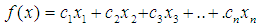 where the values of cn are real numbers and
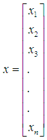 are the factors which are a compilation of the original carriable to maximize variance. It assumes these constraints and linear variables in the matrices are non-negative. If there are negative values, they must be made positive as follows [11]:
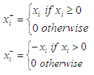 the linear regression model provides a mechanism to model the data to determine if differences between the active and inactive projects exists. For the existing sites, if the site was active, the consequence value was assigned a value of 1. If not, 0. As a result the hypothesis was that those sites likely to be successful if the SSI would tend toward a value of 1, and those that likely would not pan out, would trend toward 0. Note that because certain factors may have no value at present (example depth of an undrilled well), it is possible that the regression equation provides an SSI result that is greater than 1 or less than 0.
2.3. Further Data Manipulation
- Because the test and study site have incomplete data, the linear regression model was re-run to include only that data that would apply to the test and study sites. For example, if no well was drilled, the casing and well depths could not be known. The revised linear regression model was used to model the test and study sites to predict the likelihood of success.
3. Results and Discussion
- The states with the most ASR programs are Florida (54), followed by California, New Jersey, Arizona and Oregon (see Figure 2). However, the presence of ASR sites is not necessarily an indicator for success of ASR projects. For example, in Florida, over half the sites are not active or have wells that are no longer used. With the elimination of inactive and test sites, there are only 22 active ASR sites (as compared to 54 ASR sites) in Florida.
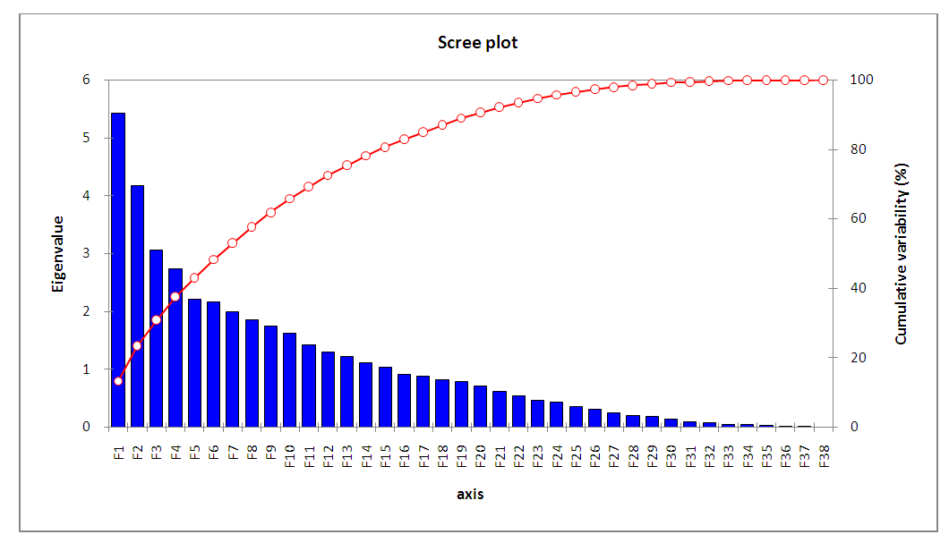 | Figure 2. Scree Plot showing that 11 factors are needed to get 70 percent of variance |
 | Table 4. Summary Statistics for Retained Variables |
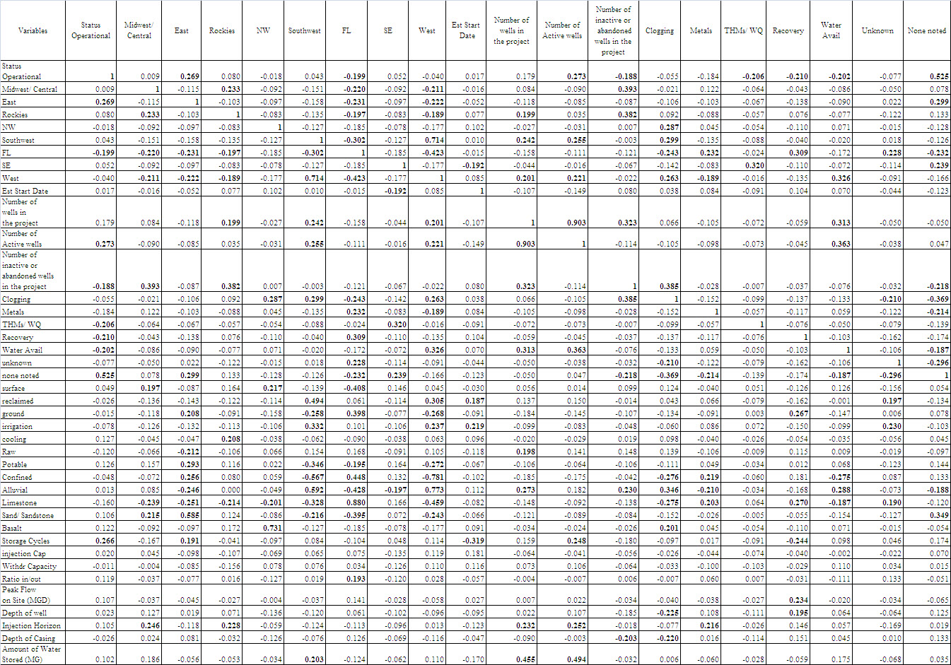 | Table 5. Correlation Analysis of retained Variables |
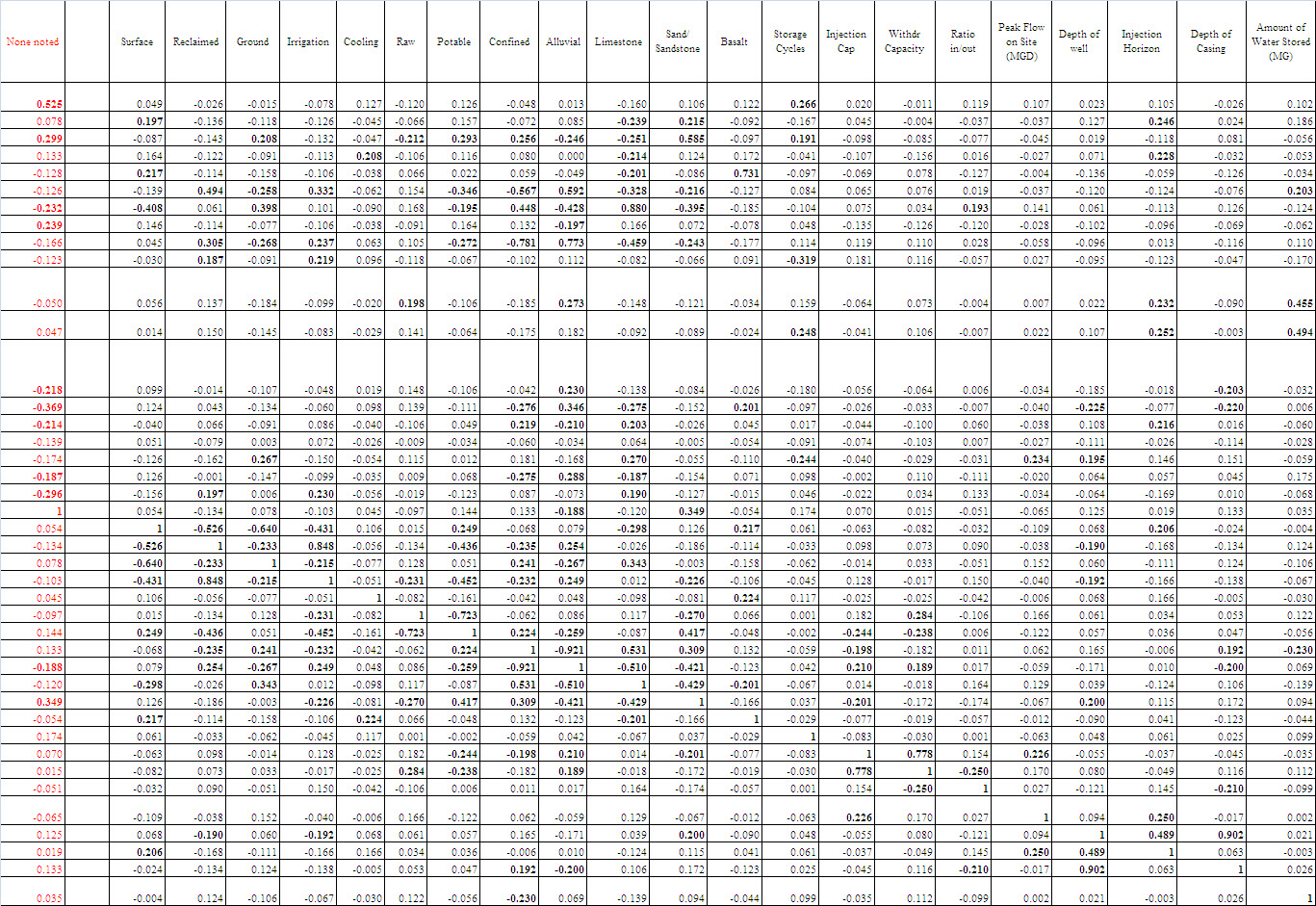 | Table 5. Continue |
 | Table 6. Factor Correlations (All 11) |
 | Table 7. Percent Contribution to the Factor |
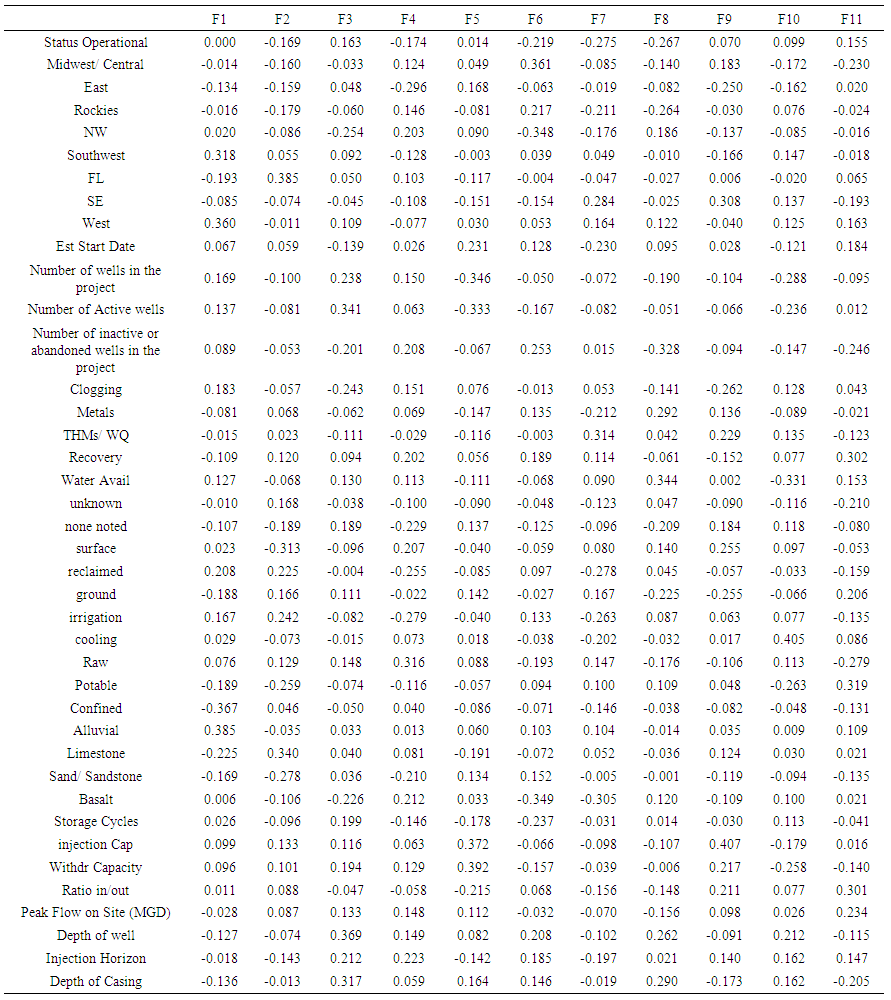
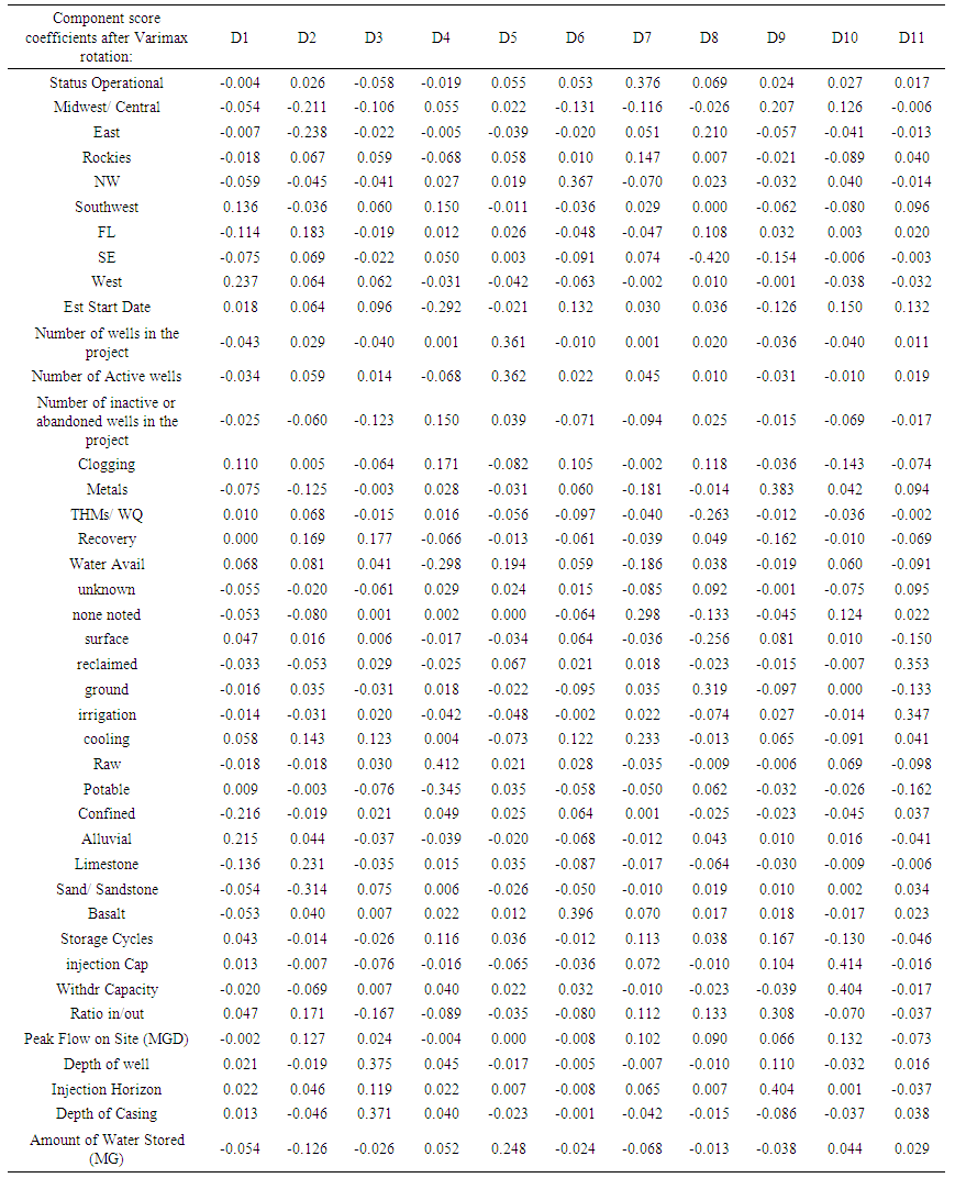 | Table 8. Factors after Varimax Rotation |
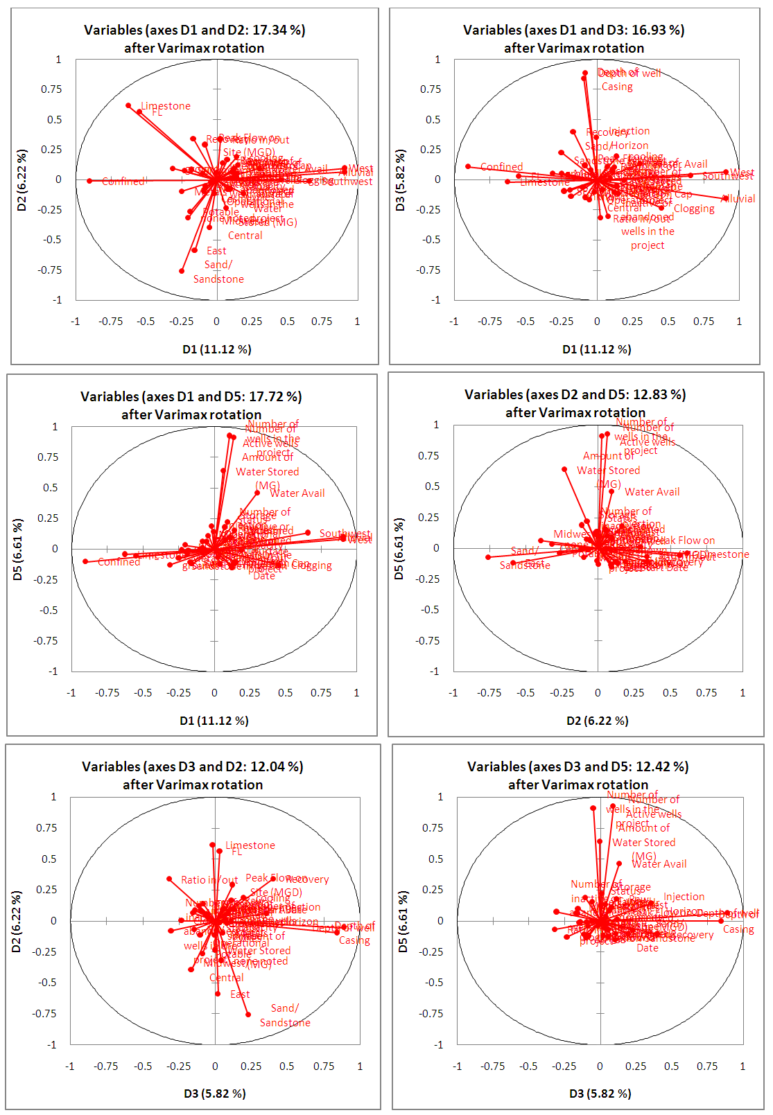 | Figure 3. Varimax Plots of Factors from PCA Analysis |
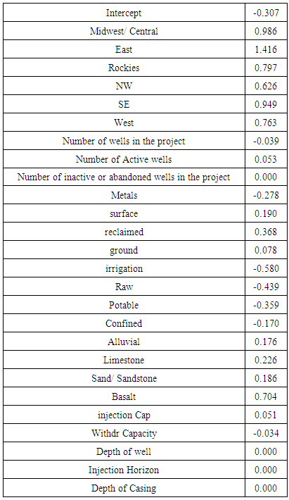
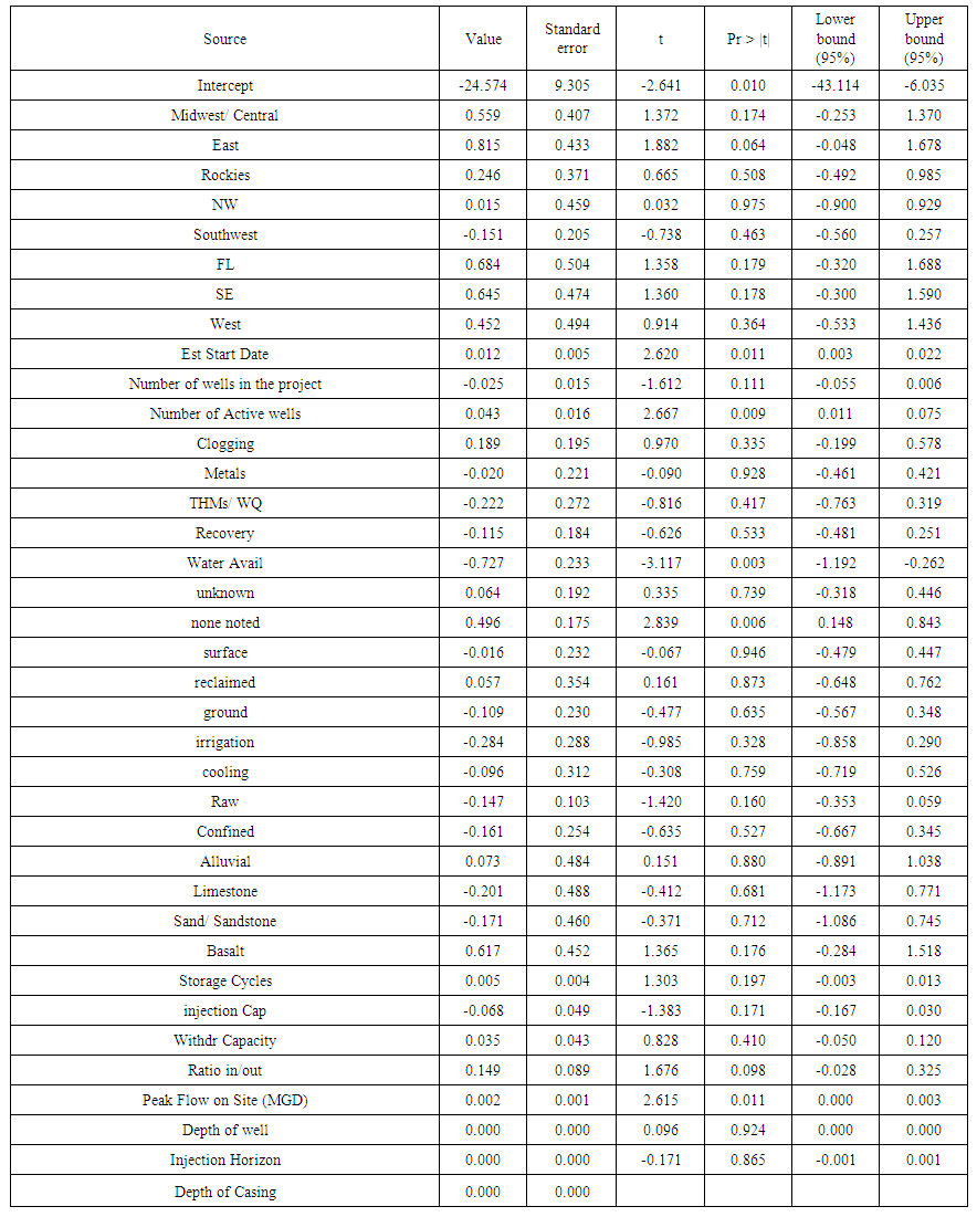 | Table 9. Linear Regression Model Parameters (all compete data for Active and inactive sites only) |
 | Table 10. Variables for the Active and Inactive Sites that also exist for the Test and Study Sites used in the revised Linear Regression model |
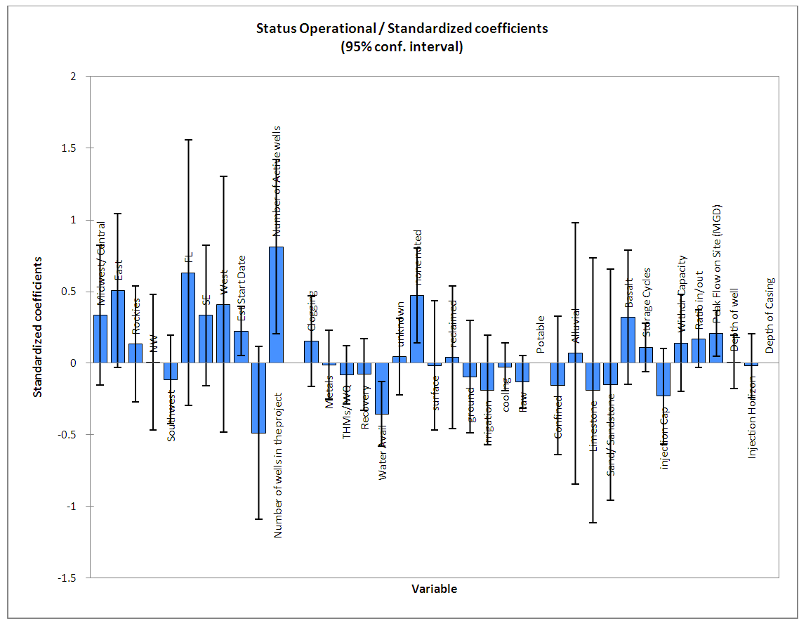 | Figure 4. Perspective on Linear Regression Model Parameters |
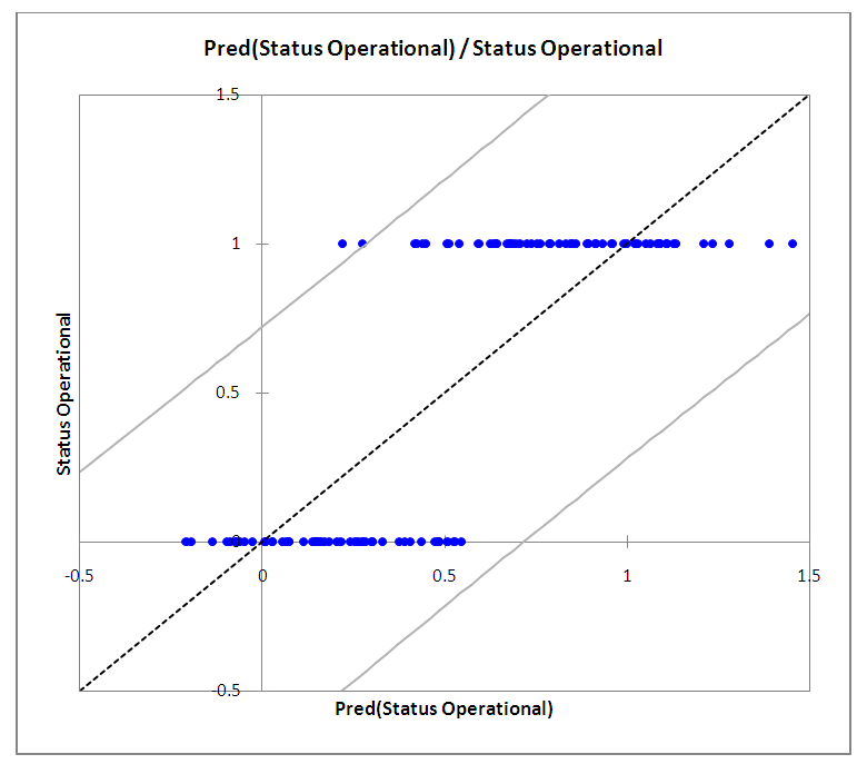 | Figure 5. Correlation between predicted and actual successful wells |
 | Table 11. Linear Regression Weights for Use in the Predictive Model |
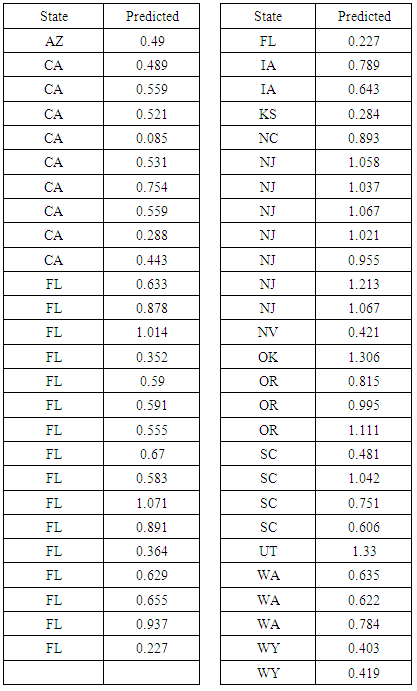 | Table 12. Summary of prediction for Success for study or Test wells |
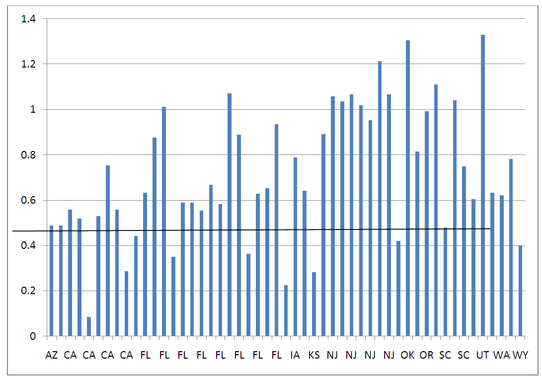 | Figure 6. Prediction on success of Test wells |
4. Conclusions
- The goal of this paper was to use this data and apply the results from active or inactive wells to those currently in the test of study phase in an effort to determine if there was a means to predict their likely success. This paper builds on the 2013 a nationwide survey of ASR systems as discussed in Bloetscher, et al [3,4] and AWWA [2]. The data from the 2013 was analyzed using factor and principal component analysis to determine correlations and variance combinations on the data. The goal was to determine which factors correlated best as a means to determine if a useful analysis could be developed to predict success of ASR systems currently in the test phase based on the success of active ASR sites.The results indicate that the use of PCA and linear regression can be used to project the potential for the test and study sites. Two thirds of the current 204 ASR sites are either active or inactive, and, once the data was sorted, 111 of those sites were able to be used to project future status. While the actual results may not be known for many years, the results shed light on the over 50 sites in this stage and their likelihood for success. The data suggests that about 1/3 of the wells have low likelihood for success and perhaps should not be pursued further.Several caveats exist for this analysis. First, the regional locations ignore that geological differences can be very different between nearby sites. Some effort was made to address this issue – for example Florida (mostly limestone) was separated from the rest of the southeast that was not. Information on salinity in the injection formation would be useful as a number of people, including the author, believe this is a major barrier to success. However, the results also suggest that more complete information would be useful for further analysis. Many sites lack full information, especially those in the study phase or are prior to 1990.