G. Degrazia, B. E. J. Bodmann, A. Wittwer, R. M. Dorado, F. Degrazia, G. Demarco, D. Roberti, A. M. Loredo-Souza, O. Azevedo, L. G. Martins
PROMEC, Federal University of Rio Grande do Sul, Porto Alegre, RS, Brazil; PPMeteorology, Federal University of Santa Maria, Santa Maria, RS, Brazil
Correspondence to: G. Degrazia, PROMEC, Federal University of Rio Grande do Sul, Porto Alegre, RS, Brazil; PPMeteorology, Federal University of Santa Maria, Santa Maria, RS, Brazil.
| Email: |  |
Copyright © 2018 The Author(s). Published by Scientific & Academic Publishing.
This work is licensed under the Creative Commons Attribution International License (CC BY).
http://creativecommons.org/licenses/by/4.0/

Abstract
The present contribution reports on the status of the STROMA experiment. As a novelty a new experimental setup in a wind tunnel allows to simulate different stability regimes with vertical heat flux in either direction. This is accomplished upon inserting a metal sheet equipped with Peltier elements into the floor of the experimental section II of the Prof. Joaquim Blessmann wind tunnel at LAC-UFRGS (Porto Alegre, Rio Grande do Sul state, Brazil). We show results and compare findings for two velocity magnitudes (1 Hz and 4 Hz) and with neutral and convective stability regime. Effects in the turbulent velocity field are presented with its dependence on height.
Keywords:
Wind Tunnel Experiment, Convective Stability Regime, STROMA experiment
Cite this paper: G. Degrazia, B. E. J. Bodmann, A. Wittwer, R. M. Dorado, F. Degrazia, G. Demarco, D. Roberti, A. M. Loredo-Souza, O. Azevedo, L. G. Martins, Wind Tunnel Experiments with Neutral and Convective Boundary Layer Stabilities, American Journal of Environmental Engineering, Vol. 8 No. 4, 2018, pp. 154-158. doi: 10.5923/j.ajee.20180804.12.
1. Introduction
The atmospheric planetary boundary layer presents still a challenge with respect to understanding its properties as well as influences of plants and buildings on wind flows, respectively. Due to a considerable complex inferior boundary, i.e. the earth’s surface, physically relevant quantities like horizontal and vertical wind speed, temperature profile and pressure, humidity distribution are subject to fluctuations that originate from a complex boundary layer dynamics. A diversity of stability regimes are a manifestation of the principal phenomenon in flows, namely turbulence. The dominant forcings are due to thermal and mechanical contributions.It is a matter of fact, that in field experiments it is hardly to encounter equal or similar boundary layer conditions. Consequently, specific experiments with comparable or compatible conditions may in principle not be reproduced. This shortcoming lead to the proposal of the present work, which is an attempt to simulate some aspects of the real planetary boundary layer in wind tunnel experiments. However, in general wind tunnel experiments are performed only in neutral stability conditions and in order to implement besides the mechanical effects also thermal contributions the test section’s floor was equipped with a aluminium sheet that was heated by Peltier elements. With such an experimental set-up it is possible to simulate the presence of a positive heat flux, which corresponds to generating a convective boundary layer comparable to a real situation.The experiment was performed in the Laboratory of Constructions Aerodynamics at the Federal University of Rio Grande do Sul, Porto Alegre, Rio Grande do Sul, Brazil. This wind tunnel is a closed return low speed wind tunnel, specifically projected for dynamic and static studies on civil construction models. Its design allows the simulation of the natural winds main characteristics. It has a length/height ratio on the main test section greater than 10 and dimensions of 1.30 m × 0.90 m × 9.32 m (width × height × length). The maximum wind speed in this chamber, with soft and uniform flow, is 42 m/s (150 km/h). The propeller is driven by an 100HP electric motor and the wind speed is controlled by a frequency inverter.The set of experiments that we report on in this work are designed to analyse and compare flows with different velocities between 1 m/s and 5 m/s for neutral and convective stability regimes, where the convective condition is driven by a temperature gradient of roughly 101K/102 mm. From the data the influence of the temperature gradient and the positive surface heat flux on the vertical profile of the flow velocity were analysed. For the accomplishment of the experiments with vertical temperature gradient two models of the test table were developed with Peltier elements, to obtain a controlled heat flux generating positive and also negative temperature gradients.
2. The Wind Tunnel Experiments
2.1. Instrumentation
In what follows are described the measuring instruments and the calibration system employed for the evaluation of boundary layer flows followed by a description of the measurements that were performed. Measurements were conducted with a hot wire anemometer (DNTEC 55P11) and the CTA System Data Acquisition System DANTEC-Stream-Line Pro (figure 1). The calibration system allows to measure the characteristics of turbulent flows subject to temperature gradients due to its temperature dependent calibration. The high time resolution allows fluctuations larger than 250 kHz. The spatial resolution allows to solve eddies with spatial scales of the order of one 1 mm (the Kolmogorov scale). Statistical parameters of turbulence are those obtained in the amplitude and frequency domain based on the time series of flow velocity. This automatic calibrator (The StreamLine Pro Automatic Calibrator) is designed to calibrate hot wire probes in air flow at very low speeds of the order of 0.5 m/s and also at high speeds up to 300 m/s.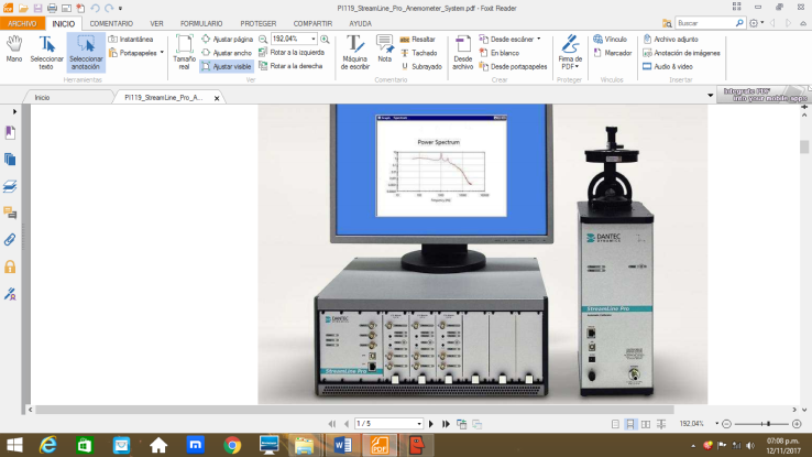 | Figure 1. Data aquisition sistem CTA System DANTEC - StreamLine Pro |
The calibration interval for measurements with low wind speed was of 0 to 101 m/s. Concomitantly, this calibrator compensates for variations in ambient temperature. During the process, the probe is located in a jet with a uniform velocity profile which is almost laminar. The calibrator is connected to a computer via USB or Ethernet, and the calibration process is controlled by the DANTEC software StreamWare Pro (see figures 2).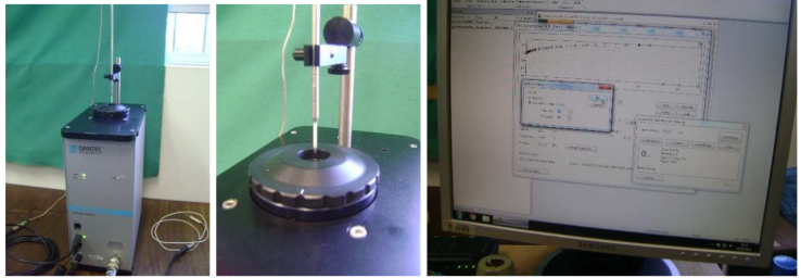 | Figure 2. Calibration system and process of an anemometer probe |
2.2. Experimental Description
The experiments were performed on table II of the wind tunnel “Prof. Joaquim Blessmann” (figure 3). From physical simulations of the boundary layer, two types of flows were evaluated; a boundary layer under neutral and unstable stability conditions, respectively. The neutral boundary layer was obtained with isothermal flow and the convective boundary layer, generated by the positive heat flux, was simulated heating the surface of table II (see figure 3). The velocity and temperature profiles (mean and variance) were acquired in the experimental section II (figure 3). The measuring points were aligned in the vertical direction and the wind profiles were obtained for 5, 10, 15, 20, 25, 30, 40, 50, 60, 70, 80, 90, 100, 150, 200, 250, and 300 mm, respectively. In this study five velocity magnitudes, corresponding to 1, 1.5, 2, 4 and 5 Hz of the speed controller of the wind tunnel were analysed. These frequencies are a variation of 1 to 5 m/s for the maximum value in each wind speed profile. At each measurement point, a time series of 368640 values was obtained with a sampling frequency of 2048 Hz. Thus, the duration of each data record was 180 s. At the same time, the records corresponding to the velocity variance and temperature at each measurement point were obtained.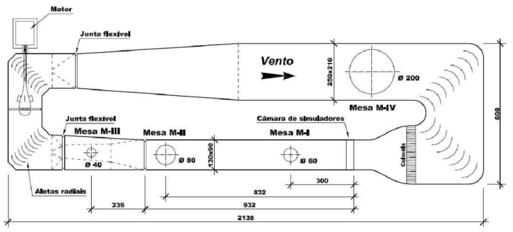 | Figure 3. Wind tunnel “Prof. Joaquim Blessmann”, LAC-UFRGS |
2.3. The Experimental Section with Peltier Elements
Two models were developed for heating or cooling the experimental section II (see figures 4). 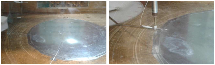 | Figure 4. Experimental section II and positioning of the hot wire anemometer |
In the first case, an aluminium sheet of 3 mm thickness and with a diameter of 800 mm, in which 12 Peltier elements (TE-127-1.4-1.5) were distributed over two circles. A smaller circle with four elements and a larger with eight elements in order to cool or heat segments of the plate with the same area. Each element had coupled a heat sink with a square section equal to the geometry of the Peltier element (4cm × 4cm × 4mm). The tests carried out showed a deficiency in heat dissipation when the plate was being cooled, that is, when the plate had the function of generating a stable boundary layer in the wind tunnel. Probably, convection and heat transfer by radiation reheated the upper sheet due to the fact of the hot side (sink) being below the cold plate. The second model, which is currently being used for the experiments, has a structure with the Peltier elements between two sheets, where the empty space in between was filled with insulation material. A sandwich structure was used for the insulating material with two aluminized polymer layers and a cork layer in between. The Peltier elements were coupled to the sheets with thermal paste (Implastec) and the two plates were fit to each other with screws of stainless steel of 3 mm diameter and 15 mm length (see figures 5). Five thermocouple (type K) were aligned radially to control the homogeneity of temperature in the sheet. The Peltier elements were connected and controlled individually by constant DC current sources (see figures 6) which allows to estimate the heat transport.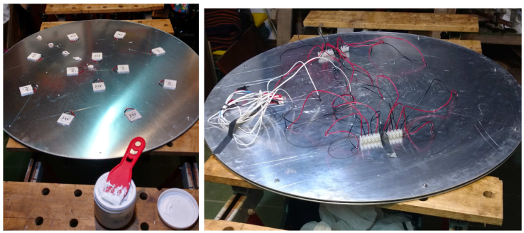 | Figure 5. Sandwich type sheet with Peltier elements, open and closed (lower sheet) |
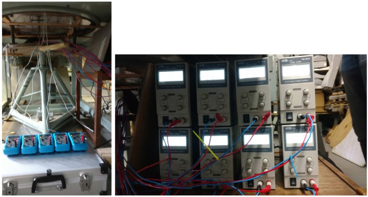 | Figure 6. Temperature control of the upper sheet (left) and power supply of the Peltier elements with constant DC current (right) |
3. Experimental Results
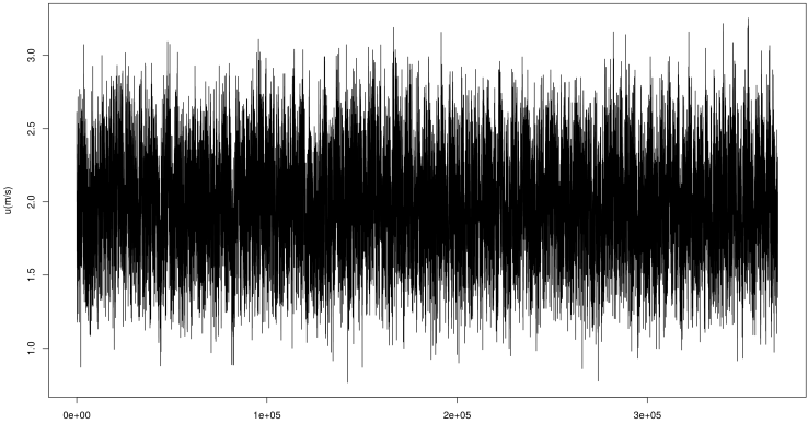
Figures 7 to 10 show the time series as measured with the hot wire anemometer. Figure 7 and 8 show the series for 1Hz at the heights z = 5 mm and z = 300 mm, respectively. At the lower position the velocity fluctuations varied between 0.10 m/s and 0.70 m/s with an average value around v = 0.45 m/s. For this case the fluctuation interval with width Δv = 0.60 m/s is larger than the average value. In other words in this height the fluctuations dominate. This changes with height so that at 300 mm the interval is located between 0.65 m/s and 0.95 m/s (Δv = 0.30 m/s) and with average velocity v = 0.81 m/s.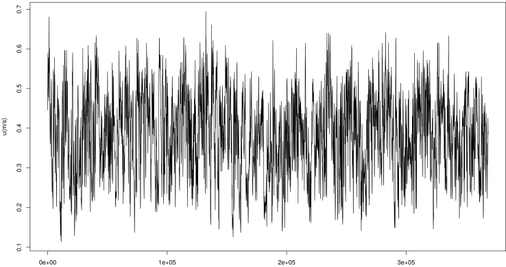 | Figure 7. Longitudinal velocity time series with 368640 sample points (equivalent to 180 s) at a height z = 5 mm and for a velocity magnitude, corresponding to 1Hz |
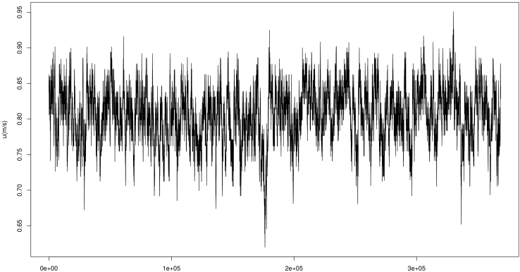 | Figure 8. Longitudinal velocity time series with 368640 sample points (equivalent to 180 s) at a height z = 300 mm and for a velocity magnitude, corresponding to 1Hz |
 | Figure 9. Longitudinal velocity time series with 368640 sample points (equivalent to 180 s) at a height z = 5 mm and for a velocity magnitude, corresponding to 4Hz |
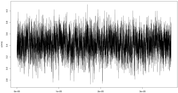 | Figure 10. Longitudinal velocity time series with 368640 sample points (equivalent to 180 s) at a height z = 300 mm and for a velocity magnitude, corresponding to 4Hz |
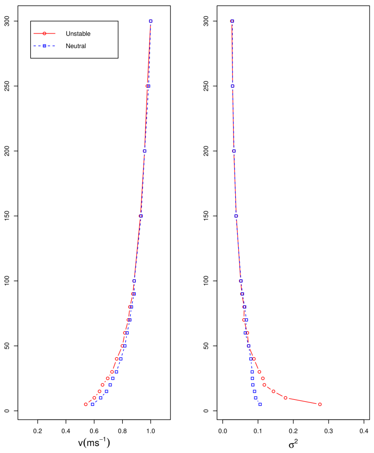
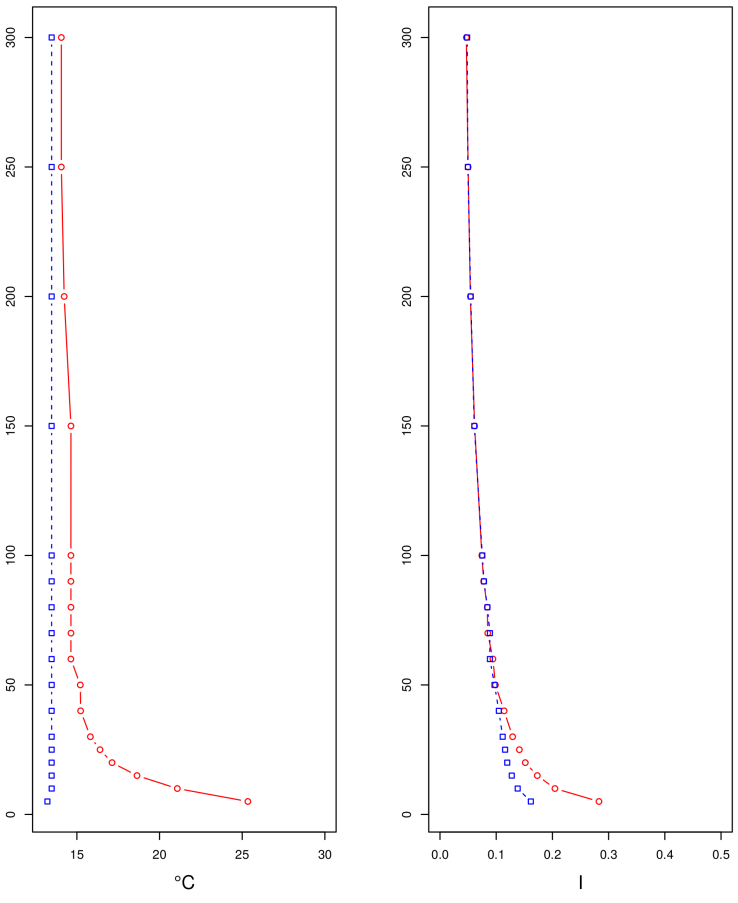
In the case of 4 Hz and the same heights as in the previous measurements the range of fluctuations at z = 5 mm are between 0.90 m/s and 3.20 m/s with a fluctuation width of Δv = 2.30 m/s, also in this case larger than the average velocity of v = 2.00 m/s. Consequently, even in the case of a larger incoming wind speed equivalent to 4 Hz, the fluctuations dominate at the position close to the floor. At z = 300 mm the fluctuation interval is between 2.80 m/s and 4.10 m/s (Δv = 1.30 m/s) and an average wind speed of 3.40 m/s. The corresponding time series are shown in figures 9 and 10, respectively.Analysis of these time series and additional measurements show the flow properties such as the vertical profile of the average velocities for the convective and neutral case. Note that velocities are normalised to the maximum velocity corresponding to the free flow (see figure 11). Further, in the same figure is also plotted the normalised variance. Comparison of the two stability cases show the effect of the vertical heat flux from below in the convective case up to a height of 100 mm. Especially, the increase of the variance is observable in agreement with increase of turbulence due to the vertical heat flow. Figures 12 show the vertical temperature profile for the two stability regimes together with the turbulence intensity, i.e. the turbulent kinetic energy. Figures 13 and 14 show the same cases for the velocity magnitude corresponding to 4Hz. From the figures one observes that the difference between the neutral and convective stability regime occurs only up to a height of 50 mm also the differences in the average velocity, variance and turbulence intensity are less than in the case with velocity magnitude corresponding to 1 Hz.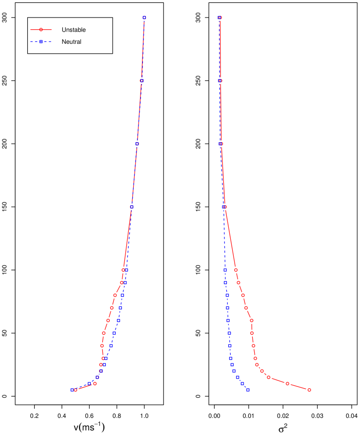 | Figure 11. Velocity and variance dependence with height z (mm) for a velocity magnitude, corresponding to 1Hz |
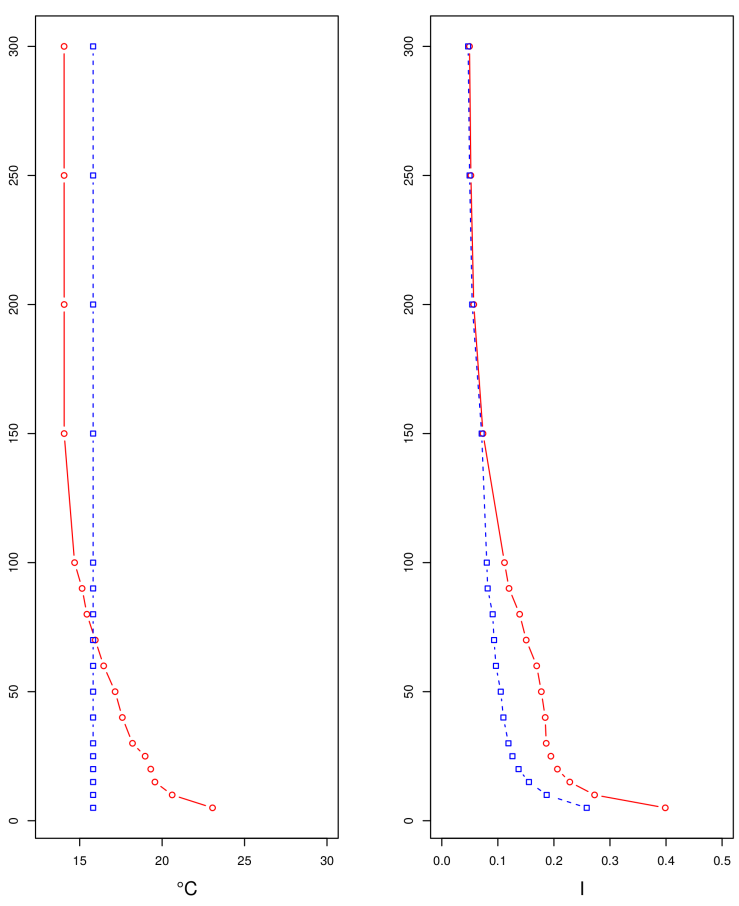 | Figure 12. Temperature and turbulence intensity dependence with height z (mm) for a velocity magnitude, corresponding to 1Hz |
 | Figure 13. Velocity and variance dependence with height z (mm) for a velocity magnitude, corresponding to 4Hz |
 | Figure 14. Temperature and turbulence intensity dependence with height z (mm) for a velocity magnitude, corresponding to 4Hz |
4. Conclusions
In the present contribution we reported on the status of the STROMA experiment, that as a novelty allows to adjust different stability regimes, i.e. besides the in wind tunnel experiments usual neutral stability also a convective regime. This is accomplished upon inserting a metal sheet equipped with Peltier elements into the floor of the experimental section II of the Prof. Joaquim Blessmann wind tunnel at LAC-UFRGS (Porto Alegre, Rio Grande do Sul state, Brazil). The Peltier elements allowed two generate a vertical temperature profile with negative gradient that resulted in a convective regime. Comparison of two velocity magnitudes of the incoming wind (1 Hz and 4 Hz) and with either neutral or convective regime showed the change in the turbulent velocity field and its dependence with height. From the data evaluation and the afore mentioned results one can claim, that the proposed setup in the wind tunnel works and that in future experiments a variety of stability regimes may be produced which opens the possibility to compare wind tunnel findings with comparable scenarios in field experiments. As next activities also a stable regime experimental run is planned with a positive temperature gradient. In a longer term we hope to gain new insights with our setup on turbulent flows, also when obstacles are placed in the flow, buildings or other objects such as wind energy generators. The first results certainly show the perspectives that arise with experiments that besides mechanical properties also allow to consider thermal effects.
ACKNOWLEDGEMENTS
The authors thank CNPq for financial support.
References
| [1] | Acevedo, Otávio C.; Mahrt, Larry; Puhales, Franciano S.; Costa, Felipe D.; Medeiros, Luiz E.; Degrazia, Gervásio A. Contrasting structures between the decoupled and coupled states of the stable boundary layer. Quarterly Journal of the Royal Meteorological Society, v. 142, p. 693-702, 2016. |
| [2] | G.A. Degrazia, H.F. Campos Velho and J.C. Carvalho, "Nonlocal exchange coefficients for the convective boundary layer derived from spectral properties", Contr. Atmos. Phys., vol. 70, pp. 57-64, 1997. |
| [3] | Puhales, Franciano Scremin; Demarco, Giuliano; Martins, Luis Gustavo Nogueira; Acevedo, Otávio Costa; Degrazia, Gervásio Annes; Welter, Guilherme Sausen; Costa, Felipe Denardin; Fisch, Gilberto Fernando; Avelar, Ana Cristina. Estimates of turbulent kinetic energy dissipation rate for a stratified flow in a wind tunnel. Physica. A (Print), v. 431, p. 175-187, 2015. |
| [4] | J.S. Irwin, "A theoretical variation of the wind profile power-low exponent as a function of surface roughness and stability", Atm. Environ., vol.13, pp. 191-194, 1979. |

 Abstract
 Reference
 Full-Text PDF
 Full-text HTML