A. S. de Athayde, L. R. Piovesan, B. E. J. Bodmann, M. T. M. B. de Vilhena
PROMEC, Federal University of Rio Grande do Sul, Porto Alegre, Brazil
Correspondence to: A. S. de Athayde, PROMEC, Federal University of Rio Grande do Sul, Porto Alegre, Brazil.
| Email: |  |
Copyright © 2018 The Author(s). Published by Scientific & Academic Publishing.
This work is licensed under the Creative Commons Attribution International License (CC BY).
http://creativecommons.org/licenses/by/4.0/

Abstract
This work presents a model where the Navier-Stokes equation is coupled to the advection-diffusion equation. The decomposition method is applied to the two-dimensional non-stationary Navier-Stokes equation and Duhamel’s Principle is used to obtain a series approximation of the solution. The concentration is represented by the Gaussian dispersion model, assuming constant diffusion coefficients.
Keywords:
Pollutant dispersion, Coupled Advection-diffusion and Navier-Stokes equation, Duhamel’s Principle
Cite this paper: A. S. de Athayde, L. R. Piovesan, B. E. J. Bodmann, M. T. M. B. de Vilhena, Analytical Solution of the Coupled Advection-Diffusion and Navier-Stokes Equation for Air Pollutant Emission Simulation, American Journal of Environmental Engineering, Vol. 8 No. 4, 2018, pp. 150-153. doi: 10.5923/j.ajee.20180804.11.
1. Introduction
The influence of the industrial revolution, technological advances and population growth has degraded nature over time. Burning of fossil fuels, deforestation, manufacturing and use of vehicles pollute and influences in the quality of air especially in large urban centres. However, humans were not alienated from this fact. To the same extent, mankind has also been using technology to study the effects of pollution and to develop appropriate physical-mathematical models to predict damages to the environment. The advancement of computers has aided in the development of numerical methods and its use has been explored on a large scale. Thus, it was possible to find approximate solutions for more complex models that cover a larger number of variables involved in the phenomenon. However, for evolution models, numerical methods require an exhaustive amount of computations to evolve from the initial condition to the desired moment and position of the model. Moreover, the boundary conditions also present several peculiarities that demand extra care. In this line, analytical methods as the GILTT (Generalized Integral Laplace Transform Technique) used in [1-3], have a considerable advantage, presenting a solution that can be calculated directly at the time and in the desired position, providing a quick answer with respect to the pollutant concentration field.In order to present a new approach to this kind of model for air pollution simulation, this work considers the main direction of the wind and the diffusion as the main responsible for transporting the pollutant through space. To this end the Navier-Stokes equation is used to represent the evolution of the wind field, coupled with the advection- diffusion equation. The two-dimensional, time-dependent Navier-Stokes equation is solved following the idea of the Adomian decomposition method [5, 6]. The basic idea is to separate the equation into a set of equations in which the non-linear advective terms are considered as the source term. The obtained equation system is then solved recursively. In each equation of the recursive system, the source term is evaluated using the solution of the previous recursion steps. In addition, the first equation of the system is subject to the initial and boundary conditions of the original problem and is solved by separation of variables. The remaining equations satisfy homogeneous boundary conditions and are solved by Duhamel’s principle [7]. The dispersion process of the pollutant is implemented by the advection-diffusion equation, and the solution used is the Gaussian dispersion model [4].The present work is organized as follows. In section 2 the mathematical model is presented, where a new technique to solve the Navier-Stokes equation is described and the gaussian solution for the advection-diffusion equation is presented. In section 3 we compare the results obtained using the proposed model with experimental data obtained in the Copenhagen experiment [11]. Finally, in section 4, we conclude and present future perspectives.
2. Coupled Advection-Diffusion and Navier-Stokes Equations
The proposed model consists of coupling a reduced version of the Navier-Stokes equation for incompressible fluids and the advection-diffusion equation, both bi- dimensional in space and time dependent: | (2.1) |
 | (2.2) |
This system is solved in a rectangular domain R = [0 L] × [0 H], where L is the longitudinal extension of the domain and H is the boundary layer height. Thus, 0 ≤ x ≤ L is the variable that represents the longitudinal distance in the main wind direction and 0 ≤ z ≤ H the height. In the above equations, u(x, z, t) denotes the wind field, u the mean wind, ν the kinetic viscosity, c(x, z, t) the mean concentration of a passive contaminant and Kx, Kz are constant diffusion coefficients. The source condition is described by a short time emission point source that is implemented by the initial condition using the Dirac delta functional, which mimics a locally concentrated pollution substance at t = 0. The boundary conditions for the wind field are considered with zero flux at ground level and the top of the boundary layer. The initial wind profile is taken as a power profile with height with a linear dependence on the distance. The solution procedure of this system is described below.
2.1. The Navier-Stokes Equation
Due to the non-linearity in the Navier-Stokes equation, there is no direct analytical solution to this equation. However, considering | (2.3) |
and following the idea of the Adomian decomposition, we replace (2.3) in (2.1) and arrange the terms to obtain the following recursive system | (2.4) |
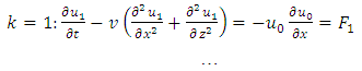 | (2.5) |
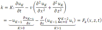 | (2.6) |
that satisfy the following initial and boundary conditions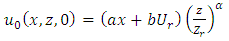 | (2.7) |
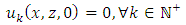 | (2.8) |
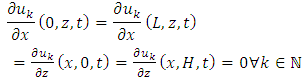 | (2.9) |
where Ur is the horizontal wind speed at a reference height Zr and α is the roughness coefficient and is related to the turbulence parameterization [8], a and b are parameters of the linear function and play the role of maintaining the power profile of the initial wind field along the main direction, but introducing a perturbation in this direction. It is noteworthy that there is a need to add a dependence in the variable x, due to the existence of the derivative in relation to this variable in the source terms Fk . However, the values of a = 10−5 and b = 1, assumed in the simulation, determine that the wind profile does not change significantly over the distance. The homogeneous equation is solved by separating variables, obtaining a series solution of the form | (2.10) |
3. Model Validation
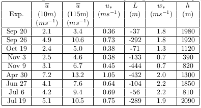
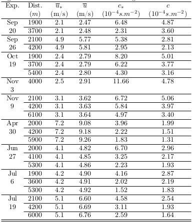
In order to validate the methodology in the previous section, the proposed solution was implemented in a computational program and a simulation of dispersion of a pollutant in the boundary layer was done in order to confront the simulated concentration values at ground level with findings from experiments.Measurements of the dispersion of a contaminant in the boundary layer consists of a sample collection sequence over a period of time. The experiment used to validate the solution was performed in the northern part of Copenhagen and is described in detail by [10-12]. Several simulations were done with different parameterizations in order to evaluate the performance of the methodology in the measurement of the contaminant. The experiment consisted in releasing SF6 from a tower 115 meters high, without buoyancy, and the sampling points were placed at ground level along three arcs. The distances between the emitting source and the collection points varied from 2 to 6 km. The emission started one hour before the sampling. The roughness length of the region was estimated 0.6 m.The average samples were collected for 1 hour with 10% imprecision. The essential data of the experiment are reported in Table 1. The experiments performed were carried out in neutral and unstable conditions according to the Pasquill stability class [8].Table 1. Meteorological condictions of the Copenhagen experiment [11] [12]
 |
| |
|
3.1. Turbulence Parameterization
In the dispersion process of pollutants, the parameterization of turbulence is crucial for meaningful results of the simulation. Due to its non-linear origin and dependency on the specific weather conditions, a considerable variety of implementations are proposed in the literature. For the model presented in this work, the parameterization chosen is based on the Taylor statistical diffusion theory and kinetic energy spectral model. This methodology, derived for convective and moderately unstable conditions, provides eddy diffusivities described in terms of the characteristic velocity and length scales of energy-containing eddies. The time dependent eddy diffusivity has been derived by [13]. However, due to the adopted simplification to consider the diffusion coefficients constant so that the solution is of Gaussian form, the diffusion coefficients were fixed and determined by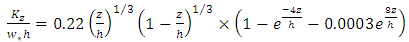 | (3.1) |
where h is the height (m) of the convective boundary layer, w∗is the vertical convective velocity (m/s). The wind speed profile (2.7) was used with the power law following the findings of the reference [8, 9].
3.2. Numerical Results
In Figure 1 one can verify convergence of the solution with increasing number of eigenvalues. Table 2, shows the results for validation, where the quantities marked with asterisk (*) are values observed in the experiment, and the ones without are values obtained by the model.All the results generated in the table were obtained by the use of 10 eigenvalues. The simulations were performed using the MATLAB R2012a software on a computer equipped with an Intel(R) Core(TM) i5-5200U CPU 2.20G processor. The time to generate the average wind and the concentration in each experiment was around 13 seconds.With 20 eigenvalues, each result would take around 596 seconds to be generated and the gain in precision would not compensate the additional CPU time. For example, in the experiment of September 26 and 2100 meters distance, the values for the mean wind and reduced concentrations would be u = 5.72 m/s and c = 2.82 × 10⁻⁴ s/m2. The increase in the number of eigenvalues increases significantly the calculation time due to the summation of products in the source term of the recursion steps. However, because the integrals of each term are calculated without numerical integration, the results are accurate and even with 10 eigenvalues the approximation already reproduces fairly well the concentrations found by experiment.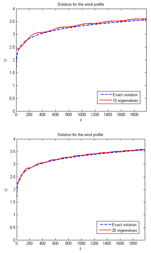 | Figure 1. Wind field at x = 0 and t = 0 for different number of eigenvalues |
Table 2. Comparison of results with those of the Copenhagen experiments [11] [12] using the initial condition based on the average wind in 10 meters
 |
| |
|
4. Conclusions
The present contribution discussed the coupled Navier- Stokes equation and the advection-diffusion equation, which allows to simulate pollutant dispersion in the planetary boundary layer in a self-consistent fashion. Thus simulations of the physical phenomenon by a solution in analytical representation were derived. The obtained solutions represent an operational tool because of its computational advantages in comparison to numerical approaches. Especially, if a phenomenon evolves with time, the need to advance in small time intervals and to take care of the stability in numerical methods may trigger an extensive amount of calculations to obtain meaningful results. Domain restrictions also require carefully chosen boundary conditions so that undesired effects do not occur that mask the results. In this sense, the analytical solutions have a great advantage, allowing for calculations for any time and position. Moreover, in the methodology used, there is almost no use of numerical integrals which allows a quick and accurate calculation of the solution terms, accelerating convergence and presenting acceptable results, even considering only few eigenvalues in the solution representation. Based on the numerical results presented, it can be observed that the methodology used generates satisfactory results from the quantitative point of view, once the order of magnitude obtained is in agreement with data from the Copenhagen experiment. In addition, the methodology is promising for implementations where the direction of the wind field varies with time, an extension that we will consider in future work.
ACKNOWLEDGEMENTS
B.E.J.B and M.T.d.V. thank CNPq for financial support.
References
| [1] | D. Buske, B. Bodmann, M.T.B. Vilhena, R. S. Quadros, "On the Solution of the Coupled Advection-Diffusion and Navier-Stokes Equations", American Journal of Environmental Engineering, vol. 5(1A), pp 1-8, 2015. |
| [2] | D.M. Moreira, M.T.B. Vilhena, D. Buske, T. Tirabassi, "The state-of-art of the GILTT method to simulate pollutant dispersion in the atmosphere", Atmospheric Research, vol. 92, pp. 1-17, 2009. |
| [3] | E.J. Silva, D. Buske, T. Tirabassi, B. Bodmann, M.T.B. Vilhena, "Modeling of Pollutant Dispersion in the Atmosphere Considering the Wind Profile and the Eddy Diffusivity Time Dependent", American Journal of Environmental Engineering, vol. 6(4A), pp. 12-19, 2016. |
| [4] | J.F. Loeck, B.E.J. Bodmann, M.T. Vilhena, "On a model for pollutant dispersion in the atmosphere with partially reflective boudary conditions", American Journal of Environmental Engineering, vol.6, pp 28-39, 2016. |
| [5] | G. Adomian, "A New Approach to Nonlinear Partial Differential Equations", J. Math. Anal. Appl., vol. 102, pp. 420-434, 1984. |
| [6] | G. Adomian, "A Review of the Decomposition Method in Applied Mathematics", J. Math. Anal. Appl., vol. 135, pp. 501-544, 1988. |
| [7] | P. Duchateau, D. Zachmann, "Applied Partial Differential Equations", Dover Publications, New York, 2002. |
| [8] | J.S. Irwin, "A theoretical variation of the wind profile power-low exponent as a function of surface roughness and stability", Atm. Environ., vol.13, pp. 191-194, 1979. |
| [9] | S.T. Roballo, G. Fisch, R.M. Girardi, "Escoamento Atmosférico no centro de lançamento de Alcântara (CLA): parte II - ensaios no túnel de vento", Revista Brasileira de Meteorologia, vol. 24, pp. 87-99, 2009. |
| [10] | S.E. Gryning, "Elevated source SF6 - Tracer dispersion experiments in the Copenhagen area", Risø-R-446, Risø National Laboratory, 187 pp, 1981. |
| [11] | S.E. Gryning and E. Luck, "Atmospheric dispersion from elevated source in an urban area: comparison between tracer experiments and model calculations". J. Appl. Meteor., vol. 23, pp. 651-654, 1984. |
| [12] | S.E. Gryning, A.A.M. Holtslag, J.S. Irwin and B. Siversten, Äpplied dispersion modelling based on meteorological scaling parameters", Atmos. Environ., vol.21, pp 79-89, 1987. |
| [13] | G.A. Degrazia, H.F. Campos Velho and J.C. Carvalho, "Nonlocal exchange coefficients for the convective boundary layer derived from spectral properties", Contr. Atmos. Phys., vol. 70, pp. 57-64, 1997. |

 Abstract
 Reference
 Full-Text PDF
 Full-text HTML