-
Paper Information
- Next Paper
- Previous Paper
- Paper Submission
-
Journal Information
- About This Journal
- Editorial Board
- Current Issue
- Archive
- Author Guidelines
- Contact Us
American Journal of Environmental Engineering
p-ISSN: 2166-4633 e-ISSN: 2166-465X
2018; 8(4): 145-149
doi:10.5923/j.ajee.20180804.10

A Sesquilinear Model Analysis for Pollutant Dispersion by the Copenhagen Experiment
 Abstract
 Reference
 Full-Text PDF
 Full-text HTML
D. L. Gisch, B. E. J. Bodmann, M. T. de Vilhena
PROMEC, Federal University of Rio Grande do Sul, Porto Alegre, RS, Brazil
Correspondence to: D. L. Gisch, PROMEC, Federal University of Rio Grande do Sul, Porto Alegre, RS, Brazil.
| Email: |  |
Copyright © 2018 The Author(s). Published by Scientific & Academic Publishing.
This work is licensed under the Creative Commons Attribution International License (CC BY).
http://creativecommons.org/licenses/by/4.0/

Dispersion of chemical agents in the atmosphere is a physical phenomenon influenced by micrometeorological variables that directly alter the dispersion behavior. The objective of a mathematical model is to aggregate information to the governing equations so that simulations reproduce a good approximation of the phenomenon. Measurements obtained through experiments help to calibrate and analyze the results obtained by mathematical models. The analytical model presented here is based on the advection-diffusion equation using Fick’s closure, whereas the concentration field is a result of a sesquilinear representation. The Copenhagen experiment was used to identify a systematics of the model parameter set with the atmospheric stability regime of the experiment.
Keywords: Pollutant dispersion, Advection-diffusion equation, Sesquilinear model
Cite this paper: D. L. Gisch, B. E. J. Bodmann, M. T. de Vilhena, A Sesquilinear Model Analysis for Pollutant Dispersion by the Copenhagen Experiment, American Journal of Environmental Engineering, Vol. 8 No. 4, 2018, pp. 145-149. doi: 10.5923/j.ajee.20180804.10.
Article Outline
1. Introduction
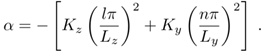
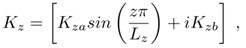
- The Kyoto Protocol from 1998, was a crucial step towards global conservation of the environment, triggering rules developments for atmospheric pollution mitigation. Currently, pollutant release into the atmosphere follows protocols requiring monitoring and adequacy in the emission limits. Each country has its own regulatory agency, such as CONAMA (Conselho Nacional do Meio Ambiente) in Brazil, which prepares laws and supervises their compliance. These agencies, following treaties and guidelines of international environmental forums, indicate the use of mathematical models as a complementary tool to estimate pollutants concentrations in industry surroundings. However, each model needs to incorporate physical and micro-meteorological characteristics compatible with each region of application.Understanding the physical phenomenon for later mathematical description is the first step in developing this monitoring tool. Thus, when observing events of pollutants dispersion, the presence of turbulent movements caused by nonlinear flow contributions has a pronounced presence. However, models for pollutant dispersion based on the advection-diffusion equation result from simplifications in order to obtain a deterministic mathematical description. This procedure eliminates the possibility of this model to reproduce turbulent characteristics fundamental for the dispersion phenomenon. Fick’s closure is an example of a formal procedure applied in the advection-diffusion equation, where the nonlinear terms, the turbulent flows, arising from the Reynolds decomposition, are replaced by a mean concentration gradient. Holmes states that nonlinear terms are essential for turbulence, and the elimination by linearization of equations weakens the results.The lack of a single mathematical definition for turbulence induces the use of some of its characteristics to describe it. The buoyancy parameter, momentum flow, and heat flow are examples of mechanisms that have structured a mathematical characterization of turbulent behavior in the equation. They generate in the dispersion phenomenon movements that form eddies, also identified as coherent structures and are a conceptual tool for reducing turbulence complexity, although there is still no unique theoretical description for them. The redefinition of the closure by a complex turbulent diffusion constant opens pathways to recover at least some of the effects induced by turbulence, i.e. by coherent structures in the present model manifest in the presence of phase differences in the solution.The vertical diffusion coefficient Kz is the ideal component to receive the phase inclusion in the advection-diffusion model, based on some already consolidated facts in mathematical models. In order to justify the choice of this component we observe the variables of the problem that are responsible for the creation of turbulent effects, such as roughness, pressure and temperature difference and daily cycle of heating and cooling of the Earth’s surface, which drive the vertical component of the phenomenon. There are also theories that attempt to overcome the lack of turbulent effects in the deterministic equations by parametrizing the turbulence for stable and convective boundary layer schemes. These models insert micro-meteorological parameters in the vertical coefficient Kz and create a profile linked to the height of the boundary layer. Thus, a phase term in the vertical component of the equation can be introduced by a complex vertical diffusion coefficient.This model recovers nonlinear effects in the system through a complex diffusion coefficient Kz introducing phase effects in the sesquilinear concentration distribution, as shown below. In proposing a new approach to advection-diffusion models with inclusion of the phase the authors are aware of the need to explore and understand its relation to the natural phenomenon. We assume that the current turbulence parameterizations applied to the vertical diffusion coefficient need calibration by experimental data in order to be applicable to real scenarios. An initial study focused on the appearance of fluctuations in the concentration distribution referring to the presence of coherent structures. Such a behaviour has never been reported in deterministic models, proving that the present modifications in the advection-diffusion equation and the resulting concentration representation comes closer to the physical description of the phenomenon. We also showed that the variation in the parameter responsible for the phase presence generates different fluctuation patterns in the concentration distributions, besides contributing to the dispersion characteristics of the pollutant. In this work we present a relation of the present model to the data from the Copenhagen experiment, which has low, moderate and high turbulent convective regimes. By simulating the experiment by this model it is possible to show that there are semi-quantitative evidences that the ratio of real to the imaginary part of the turbulence diffusion coefficient relates to the afore mentioned stability regimes.
2. The Advection-Diffusion Equation and New Closure
- The pollutants dispersion models is based in the advection-difusion equation [13, p. 131]
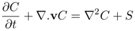 | (1) |
 | (2) |
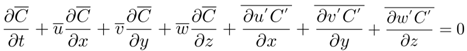 | (3) |
 and
and  are known as turbulent flows. Solving now the equation analytically requires replacing them here by a modified Fick’s closure [7], i.e. the turbulent flows will be replaced by concentration gradients and a phase is introduced into the vertical diffusion coefficient Kz through a complex paramater in comparison to the traditional Fick closure [15]. Thus the equation of the model, with wind velocity in the x direction is given by
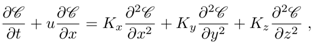 | (4) |
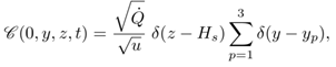 | (5) |
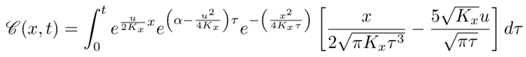
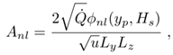
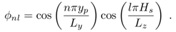
 [g/s], the coordinate of the source along the y axis is yp [m] and height is given by Hs [m], respectively. The three sources are at the same height and located at x = 0, with coordinates y in 0.1, 0, and −0.1 m. The flux of pollutants is considered null at the boundaries of a domain with dimensions Lx , Ly and Lz. The techniques used to obtain the solution are the separation of variables, using a Sturm-Liouville procedure in the directions y and z and the Laplace transform in x and also t.The model’s solution is given in sesquilinear form
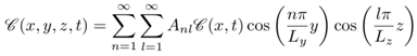 | (6) |
 | (7) |
 | (8) |
 | (9) |
 | (10) |
 | (11) |
3. Model Validation
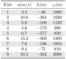
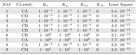
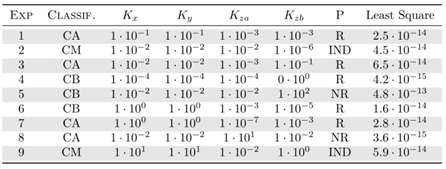
- The sesquilinear model is used now to simulate the Copenhagen experiment described in detail in reference [12]. The series of experiments provide runs in three stability regimes, classified by a criterion [17] where a ratio between the convective boundary layer height and the Monin-Obukhov length determine the type of test convection. A tracer substance sulphurhexafluoride (SF6) was released without buoyancy from a 115-meter-high source at a constant flow rate ranging from 2.4 to 4.7 g/s and release time interval of 60 minutes. Measurements were taken at ground level where the terrain roughness is taken into consideration, being an urban region, that is, z0 = 0.6 meters. Up to three series of samples were collected for each test and positioned between 2 to 6 km from the release location. In this work we analyzed only the maximum concentration values obtained in the measurements of the 9 experiments [18]. The parameter used in the model are presented in table 1.
|
 | (12) |
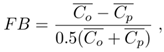 | (13) |
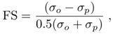 | (14) |
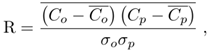 | (15) |
4. Results
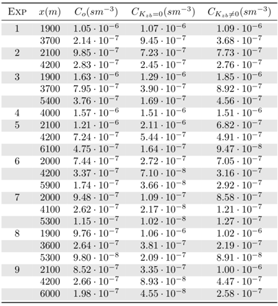
- The approach in the advection-diffusion model with modified Fick’s closure allowed to show correlations between a complex turbulent diffusion parameter (the presence of a phase) in the vertical diffusion coefficient. Recalling that the vertical coordinate is highly associated with the existence of turbulent processes in the atmosphere, variation of roughness, momentum, heat exchanges by soil irradiation and temperature gradient justifies the attempt to implement the proposed modification in the vertical component only.The sesquilinear model concentration distributions do not show fluctuations in cases where the phase is equal to zero Kzb = 0, where the original deterministic model is recovered. Fluctuations in general arise for complex coefficients whose imaginary part is nonzero [10]. The concentration distributions that have fluctuations were evaluated by independent variation of parameters in the real and imaginary part of the vertical coefficient and the result is presented in figure 1.
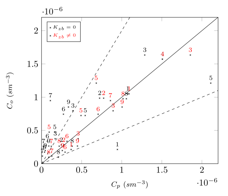 | Figure 1. Scatter plot for predicted (Cp) observed (Co) concentrations for the simulations of the Copenhagen experiment without the phase (Kzb = 0) in black and with the phase (Kzb ≠ 0) in red. The number represents the respective experiment the data are taken from |
|
|
|
5. Conclusions
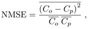
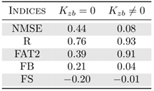
- The advection-diffusion model with complex closure and sesqui-linear pollution concentration showed to be able to identify a semi-quantitative pattern for different stability regimes, which added to previously obtained results, confirms again its promising potential. The behavior of the sesqui-linear model shows local fluctuations in the concentration field which is also observed in field experiments. With decreasing stability in the planetary boundary layer the agreement between model predictions and experimental data was achieved by increasing contributions of an imaginary turbulent diffusion coefficient. A model inherent effect is that also the intensity of fluctuations in the density of concentrations increases. These findings were obtained as a result using the minimum square value, confirmed by the scatter plot, and are accompanied by a significant improvement of the statistical indices. Nevertheless, the model needs to be studied and calibrated with micro-meteorological parameters, since we showed sensitivity to changes in the stability regime.
ACKNOWLEDGEMENTS
- This work was supported by Linhares Geração SA, Tevisa, CAPES - Brazil and CNPq - Brazil.
References
| [1] | P. Holmes, J. L. Lumley, and G. Berkooz, Turbulence, Coherent Structures, Dynamical Systems and Symmetry. Cambridge Monographs on Mechanics, Cambridge University Press, 1996. |
| [2] | S. Möller and J. H. Silvestrini, “Turbulência: fundamentos,” in Turbulência, vol. 4, ch. 1, p. 32, Associação Brasileira de Engenharia e Ciências Mecânica, 2004. |
| [3] | H. J. S. Fernando, Handbook of Environmental Fluid Dynamics II. CRC press, 2013. |
| [4] | C. Tropea, A. L. Yarin, and J. F. Foss, Springer handbook of experimental fluid mechanics. No. 1, Springer Berlin Heidelberg, 2007. |
| [5] | G. A. Degrazia, H. F. C. Velho, and J. C. Carvalho, “Nonlocal exchange coefficients for the convective boundary layer derived from spectral properties,” Contributions to Atmospheric Physics, vol. 70, pp. 57–64, 1997. |
| [6] | G. A. Degrazia, M. T. Vilhena, and O. L. L. Moraes, “An algebraic expression for the eddy diffusivities in the stable boundary layer: a description of near-source diffusion,” Il Nuovo Cimento, vol. 19C, pp. 399–403, 1996. |
| [7] | D. L. Gisch, B. E. J. Bodmann, and M. T. B. Vilhena, Two Reasons Why Pollution Dispersion Modeling Needs Sesquilinear Forms, ch. 22, pp. 257–266. Cham: Springer International Publishing, 2015. |
| [8] | G. A. Degrazia and O. L. L. Moraes, “A model for eddy diffusivity in a stable boundary layer,” Boundary-Layer Meteorology, vol. 58, no. 3, pp. 205–214, 1992. |
| [9] | G. A. Degrazia, D. M. Moreira, and M. T. Vilhena, “Derivation of an Eddy Diffusivity Depending on Source Distance for Vertically Inhomogeneous Turbulence in a Convective Boundary Layer,” Journal of Applied Meteorology, vol. 40, pp. 1233–1240, jul 2001. |
| [10] | D. L. Gisch, B. E. J. Bodmann, and M. T. M. B. Vilhena, “A Genuine Solution of the Diffusion Advection Equation Sesquilinear Way to Multi-Source Problem,” American Journal of Environmental Engineering, vol. 6, pp. 160–163, 2016. |
| [11] | D. L. Gisch, B. E. J. Bodmann, and M. T. M. B. Vilhena, “Analytical Model Study for the Pollutants Dispersion with Coherent Structures Presence,” Proceeding Series of the Brazilian Society of Applied and Computational Mathematics, vol. 6, no. 1, 2018. |
| [12] | S. E. Gryning, Elevated Source SF 6 -Tracer Dispersion Experiments in the Copenhagen Area. Denmark: Risoc National Laboratory, Roskilde, 1981. |
| [13] | S. P. Arya, Air Pollution Meteorology and Dispersion. New York, USA: Oxford University Press, 1999. |
| [14] | R. B. Stull, An Introduction to Boundary Layer Meteorology. Dordrecht, Holanda: Kluwer Academic Publishers, 1988. |
| [15] | J. Daily and D. Harleman, Fluid Dynamics. Mass., USA: Addison-Wesley Publishing Company, 1966. |
| [16] | J. D. Jackson, Classical electrodynamics. New York, NY: Wiley, 3rd ed., 1998. |
| [17] | H. A. Panofsky and J. A. Dutton, Atmospheric Turbulence. New York: John Wiley & Sons, 1984. |
| [18] | S. E. Gryning and E. Lyck, “Atmospheric dispersion from elevated sources in an urban area: Comparison between tracer experiments and model calculations,” Journal of Climate and Applied Meteorology, vol. 23, no. 4, pp. 651–660, 1984. |
| [19] | S. R. Hanna, “Confidence limit for air quality models as estimated by boot-strap and jacknife resampling methods,” Atmospheric Environment, vol. 23, pp. 1385–1395, 1989. |