Tiziano Tirabassi1, Daniela Buske2
1Università Politecnica delle Marche, Italy and Universidade Federal de Santa Maria, Brasil
2Programa de Pós-Graduação em Modelagem Matemática, Universidade Federal de Pelotas, Pelotas, Brasil
Correspondence to: Tiziano Tirabassi, Università Politecnica delle Marche, Italy and Universidade Federal de Santa Maria, Brasil.
| Email: |  |
Copyright © 2018 The Author(s). Published by Scientific & Academic Publishing.
This work is licensed under the Creative Commons Attribution International License (CC BY).
http://creativecommons.org/licenses/by/4.0/

Abstract
After setting a realistic scenario of the Atmospheric Boundary Layer (ABL), through the wind and diffusivity parameterizations, an explicit approximate expression is provided for the ground level concentration, allowing an analytic simple expression for the position and value of the maximum concentration, that results as an explicit function of the parameters defining the ABL scenario and the source height. The proposed formula is useful as an additional tool for decisional as well as emergency responses.
Keywords:
Air pollution modelling, Analytical solutions, Advection-diffusion equation, Maximum concentration
Cite this paper: Tiziano Tirabassi, Daniela Buske, An Operative Formula for the Maximum Ground Level Concentration from a Point Source, American Journal of Environmental Engineering, Vol. 8 No. 4, 2018, pp. 140-144. doi: 10.5923/j.ajee.20180804.09.
1. Introduction
The management and safeguard of air quality presupposes a knowledge of the state of the environment. Such knowledge involves both cognitive and interpretative aspects. Monitoring networks and measurements in general, together with an inventory of emission sources, are of fundamental importance for the construction of the cognitive picture, but not the interpretative one. In fact, air quality control requires interpretative tools that are able to extrapolate in space and time the values measured by analytical instrumentation at field sites, while environmental improvement can only be obtained by means of a systematic planning of reduction of emissions, and, therefore, by employing instruments (such as mathematical models of atmospheric dispersion) capable of linking the causes (sources) of pollution with the respective effects (pollutant concentrations).The processes governing the transport and diffusion of pollutants are numerous, and of such complexity that it would be impossible to describe them without the use of mathematical models. Such models therefore constitute an indispensable technical instrument of air quality management.Moreover, in cases of environmental accidents or even catastrophes one needs fast procedures, which yield immediate results as for instance the ground level concentration of pollutants, especially the maximum concentration and its position. Numerical simulation approaches may still be too slow to provide a map of concentrations in real time, when immediate decisions are necessary. The computational evaluation of numerical data of the concentration field or for a set of position have to be an instant task. In this line the present work presents a derivation of compact phenomenological formula extracted from the analytical GILTT (Generalized Integral Laplace Transform Technique) approach [1] which permits to determinate quickly the ground level concentration in terms of physical parameters.This paper is divided into six sections. In the following sections, the analytical solution of the advection-diffusion equation (ADE) and the turbulent parameterization used are presented. In section 4 the ground level concentration is obtained. Finally, sections 5 and 6 are reserved for the results and conclusions, respectively.
2. The ADE Solution
The crosswind integration of the ADE (in stationary conditions and neglecting the longitudinal diffusion) leads to: 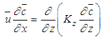 | (1) |
for  and
and  , subject to the boundary conditions
 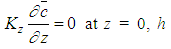 | (1a) |
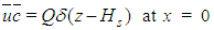 | (1b) |
with h the top of ABL, Q the emission rate at height Hs and δ the generalized Dirac delta functionFollowing the work [1], we pose that the solution of problem (1) has the form: 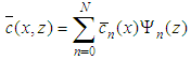 | (2) |
where  are the eigenfunctions of the associated Sturm-Liouville problem, we mean,
  where
where  (n=0,1,2,…) are the respective eigenvalues. To determine the unknown coefficient
  we replace Eq. (2) in Eq. (1) and applying the operator
  , we come out with the result in matrix form:
  | (3) |
Here Y(x) is the vector whose components are  and
and  ;
;  and
and  are the matrices whose entries are respectively
  and
and .The source condition for the transformed problem (3) is obtained from Eq. (1b), and given by
 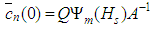 , where A-1 is the inverse matrix of A given by
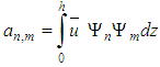 .The transformed problem represented by the Eq. (3) is solved analytically, combining Laplace transform technique and diagonalization of the matrix F . After some algebra, we come out with the result:
 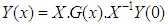 | (4) |
where X is the matrix of the eigenvectors of the matrix F and X-1 it is the inverse. G(x) is a diagonal matrix with components  (dn are the eigenvalues of the matrix diagonalization). Once
  , the final two-dimensional solution of problem (1) is determined by Eq. (2).
3. Turbulent Parameterization
The choice of the turbulent parameterization is set to account for the dynamics processes occurring in the ABL. In the further we restrict our discussion to simple vertical profiles of wind and eddy diffusivity, nevertheless still reasonably realistic, more specifically unstable regime. For an extension including stable regimens we refer to a future work. The choice of the vertical profile for the wind  is set to be following a power law [2]:
 | (5) |
where  is the mean wind velocity at the height z1, while α is an exponent related to the turbulence intensity [3]. On the quantitative side, results will be provided setting α = 0.1, and the reference wind u1(0.01h) = 3ms-1; these values are quite consistent with the whole range of unstable regimes pointed out by [4].The vertical diffusivity parameterization is chosen according to [5], which for an unstable ABL it is given as:
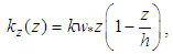 | (6) |
where h is the height of the ABL, k is the von Karman constant which is set to 0.4, and w* is the convective scaling parameter related to the Monin-Obukhov length LMO and the mechanical friction parameter u* as: | (7) |
For convective scenarios LMO is limited to values such that the relationship h / LMO < -10 holds. Finally, u* is determined as [2, 6]  | (8) |
where z0 is the roughness (10-5 h). For an unstable ABL, ψ is defined as  and
and  .The chosen profiles ensure simple functions and still rather realistic horizontal wind
  and turbulent eddy diffusivity Kz inside and both edges of the ABL.
4. Ground Level Concentration
Ground Level Concentration (GLC will be reported in terms of the dimensionless GLC as follows: | (9) |
where  is the vertically averaged wind introduced in Eq. (5)
 | (10) |
If we consider the definition of  profile in Eq. (5) we have
  .Definition (9) has been introduced to obtain the unitary limit independent of a specific parameter choice
  , according to the theoretical expectation for the two-dimensional ADE solution.In [7, 8] the GILTT results are compared with experimental data. The scope of this paper is to provide a simple explicit expression for the maximum GLC,
  , occurring at the horizontal distance
  as a function of the setting parameters for ABL scenario and source emission. As previously mentioned, in fact, although the sum (2) represents the exact solution of the Eq. (1), except for a round-off error, the series expansion misses manifest dependencies on ABL parameters and source height. Then the core of the problem leads to investigate on the behaviour of the series (2) after setting z = 0, and using the property of the Sturm-Liouville eigenfunctions for which
  regardless the index i. An analysis of the behaviour and properties of the series (2) shall indicate how to synthesize the considerable expression into a more compact formula. The results based on such an approach are still profile depending. Nevertheless, the choice of a profile depending approximation still maintains the advantage of simplicity and permits for a specific case to explore the functional behaviours of the main physical parameters that drive atmospheric diffusion. So, we introduce empirical parameters which are determined by fit procedures to best reproduce the exact solution.Based on these facts, and being in mind the Gaussian solution and the GLC obtained with power low profile of wind and eddy diffusivity [9, 10], the dimensionless GLC defined in Eq. (9) can be approximated as follows:
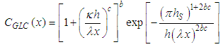 | (11) |
Due to the negative values assumed by the Monin-Obukhov length, in the following it will be defined as the positive dimensionless parameter 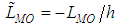 . Parameters b, c, κ and λ have been determined by least squares fittings procedures on Eq. (11) against the analytical solution and these result:
 | (12) |
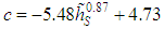 | (13) |
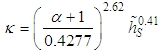 | (14) |
 | (15) |
where the variables with  are normalized with respect to the ABL height h (e.g.
  ).Equations (12) – (15) give the explicit dependency on the source height hs, the wind parameters α (it compares in k and λ),
  and the convection scaling parameter w* (it compares in λ¸ see Eq. (15)) which is related to the Monin-Obukhov length LMO and the friction parameter u* by the relationship (7). Some considerations about the parameters b and c. The approximation of Eq. (11) reduces to the simple Gaussian GLC when b and c are such that bc = 0.5. In Figure 1 is shown the product bc versus hs, where for
  reaches
  , which is the closest value to the Gaussian solution value (0.5). It is worth to remind that the eddy diffusivity (6) is symmetric in respect of the middle of the ABL. The product tends to 0.5+ when turbulence reduces, meaning for this couple of parameters a dependency on LMO. Nonetheless such a dependency is always negligible compared to the dependence on hs, the λ parameter turbulence dependency compensates such a missing. Away from the ABL middle and for low sources bc ≈ 0.8 due to the high z-gradient on
  and Kz.
  | Figure 1. A scan of the product bc versus the source height hs/h |
To confirm the goodness of the approximation, in Figures 2(a-c) the GLC versus  is shown for three
  . For each source height two extreme Monin-Obukhov lengths are used with
  = 0.001, 0.099 (empty squares and triangles respectively). The second value for
  reflects the limit imposed by the eddy diffusivity given by Eq. (6). The GILTT-based GLC are superimposed on the approximation of Eq. (11) (dotted lines). Plots show that for near surface sources there is a slight difference between points and lines near the source position, where the horizontal gradient is most pronounced (a logarithmic scale enhance such a discrepancy), nonetheless, the GILTT results are reproduced fairly well in the area of maximum concentration.From the explicit approximation for
  one may evaluate the position where the maximum for GLC occurs, in fact putting equal to 0 the derivative of Eq. (11) in respect to x and with the assumption that:
  | (16) |
 | Figure 2. GLC versus  for (a) for (a)  , (b) , (b)  , and (c) , and (c)  . Points refer to the GILTT results, dotted lines to the approximation function of Eq. (11) . Points refer to the GILTT results, dotted lines to the approximation function of Eq. (11) |
we have: | (17) |
Finally, putting  in Eq. (11), the corresponding Maximum Ground Level Concentration
  is:
is: | (18) |
The expression for the position  is valid provided that in the range of horizontal distances where a position
  occurs. Such approximation affects an error when high sources are concerned, indeed above
  , but high convection driven turbulence enforces condition (16).
5. Results
Figures 3 and 4 show plots of the maximum GLC  and its position
  for several source height
  and for a selection of turbulence parameter
  . In both figures the GILTT results (points) are superimposed on the approximations (17) (dotted lines).
  | Figure 3. Position of the maximum GLC versus the source height  . Points refer to the GILTT results, dotted lines refer to Eq. (17) . Points refer to the GILTT results, dotted lines refer to Eq. (17) |
 | Figure 4. Value of the maximum GLC versus the source height  . Points refer to the GILTT results, dotted lines refer to Eq. (18) . Points refer to the GILTT results, dotted lines refer to Eq. (18) |
Figure 3 depicts the position where the maximum occurs, where GILTT results (dotted lines) and our approximations (solid lines) show good matching regardless the turbulence regime. The turbulence dependency shows that for a fixed  the strength of convection causes
  to get closer to the source. From the physics point of view this result agrees with the mixing effect of turbulence.A final remark should be made about Figure 4. Both GILTT and expression (18) confirm that the maximum GLC value depends on the source height, regardless the turbulence. Based on the expression (18) and the parameters definitions (12)-(15), for b, c and
  , the leading term for the maximum GLC results:
 | (19) |
where the exponent -1 is a lower bound for the source term. These results broaden the well-known result obtained with the Gaussian approach for an unbounded ABL. Furthermore, this agrees with the two-dimensional Gaussian result that the maximum for the GLC is: | (20) |
6. Conclusions
The results presented in this paper have shown the possibility to express the GLC from an emitting point source in a steady convective ABL, by a compact analytical expression. The function was determined analysing the behaviour of the series expansion provided by the GILTT solution. Despite the simplifications due to restricting to only unstable ABL regimes, the analysis allows to understand to a high extent the form of the ground level concentration.The principal progresses worth emphasizing is that for a function given in (11), within the setting choice for the ABL parameter set, the maximum GLC depends only on the source height, regardless the Monin-Obukhov length. On the other hand, turbulence can still affect the position where the maximum GLC occurs, which is also confirmed by the GILTT solution. On the operative point of view, the expression (11) and its related features are useful as an additional tool for decisional as well as emergency responses.
ACKNOWLEDGEMENTS
The authors thank CNPq (Conselho Nacional de Desenvolvimento Científico e Tecnológico) and Regione Marche - Italy for the partial financial support of this work.
References
| [1] | Moreira D.M., Vilhena M.T., Buske D., Tirabassi T., 2009, The state-of-art of the GILTT method to simulate pollutant dispersion in the atmosphere, Atmospheric Research, 92 (1), 1-17. |
| [2] | H. A. Panofsky, J. A. Dutton, Atmospheric Turbulence, New York: John Wiley & Sons, 1988. |
| [3] | Irwin, J.S., 1979, A theoretical variation of the wind profile power-low exponent as a function of surface roughness and stability, Atmos. Environ., 13, 191-194. |
| [4] | F. Pasquill, F. B. Smith, Atmospheric Diffusion, New York: John Wiley & Sons, 1984. |
| [5] | Pleim, J. E., Chang, J. S., 1992, A nonlocal closure.model for vertical mixing in the convective boundary-layer. Part A-General Topics, Atmos. Environ., 26, 965-981. |
| [6] | P. Zannetti, Air Pollution Modelling, Computational Mechanics Publications, Southampton, 444pp, 1990. |
| [7] | Moreira, D. M., Vilhena, M. T., Buske, D., Tirabassi, T., 2006, The GILTT solution of the advection-diffusion equation for an inhomogeneous and nonstationary ABL, Atmos. Environ., 40, 3186-3194. |
| [8] | Buske, D., Vilhena, M. T., Moreira, D. M., Tirabassi, T., 2007, Simulation of pollutant dispersion for low wind conditions in stable and convective planetary boundary layer, Atmos. Environ., 41, 5496-5501. |
| [9] | Tirabassi, T., 1989, Analytical air pollution advection and diffusion models, WASP, 47 (1-2), 19-24. |
| [10] | Tirabassi, T., 2003, Operational advanced air pollution modelling, PAGEOPH, 160 (1-2), 5-16. |

 Abstract
 Reference
 Full-Text PDF
 Full-text HTML