-
Paper Information
- Next Paper
- Previous Paper
- Paper Submission
-
Journal Information
- About This Journal
- Editorial Board
- Current Issue
- Archive
- Author Guidelines
- Contact Us
American Journal of Environmental Engineering
p-ISSN: 2166-4633 e-ISSN: 2166-465X
2018; 8(4): 135-139
doi:10.5923/j.ajee.20180804.08

Analytical Model for Dispersion of Rocket Exhaust – Source Size Impact Assessment
 Abstract
 Reference
 Full-Text PDF
 Full-text HTML
Bruno K. Bainy1, Bardo E. J. Bodmann2, Daniela Buske3, Régis Quadros3
1Department of Meteorology, Federal University of Pelotas, Pelotas, Brazil
2Department of Mechanical Engineering, Federal University of Rio Grande do Sul, Porto Alegre, Brazil
3Department Mathematics and Statistics, Federal University of Pelotas, Pelotas, Brazil
Correspondence to: Bruno K. Bainy, Department of Meteorology, Federal University of Pelotas, Pelotas, Brazil.
| Email: |  |
Copyright © 2018 The Author(s). Published by Scientific & Academic Publishing.
This work is licensed under the Creative Commons Attribution International License (CC BY).
http://creativecommons.org/licenses/by/4.0/

This work presents sensitivity tests of a model for calculation of rocket effluent dispersion, with respect to the source size. The model employs the Generalized Integral Laplace Transform Technique (GILTT) to solve, analytically, the advection – diffusion equation. By employing different virtual sources, the point source was changed into volume sources with previously defined crosswind radius (0, 10, 25 and 50 m), and the impact of such modification was assessed in terms of the vertical distribution of atmospheric contaminants and the concentration fields close to the surface. The tests were conducted for cases of stable and unstable planetary boundary layer.
Keywords: GILTT, Pollution dispersion, Volume source
Cite this paper: Bruno K. Bainy, Bardo E. J. Bodmann, Daniela Buske, Régis Quadros, Analytical Model for Dispersion of Rocket Exhaust – Source Size Impact Assessment, American Journal of Environmental Engineering, Vol. 8 No. 4, 2018, pp. 135-139. doi: 10.5923/j.ajee.20180804.08.
Article Outline
1. Introduction
- The process of launching spacecrafts starts with the ignition, in which the vehicle acquires thrust for a few seconds, followed by the removal of the launching platform, and by leading it to its trajectory. In these first seconds, there is a massive emission of pollutants that are released towards the ground, forming a large, hot and highly toxic cloud. This cloud is called ground cloud and, due to its thermodynamics characteristics, ascend through the troposphere until it reached thermal equilibrium with the environment. The ground cloud is, generally, the object of special interest in what concerns potential risks to human health and safety [1].Aiming the protection of rockets launching sites, as well as of the inhabitants and sojourners, fauna and flora of the regions adjacent to those sites, it is necessary the use of modelling the dispersion of the emitted contaminants prior to the launching itself, so that the dispersion conditions can be assessed, and the exposure safety criteria can be met. However, because of the high complexity of the processes of formation, ascension, and dispersion of the ground cloud, many considerations and assumptions have been made to simplify the physical problem to solve it. Numerical modelling usually present advantages in terms of the physical representation and increased details regarding the atmospheric conditions and chemical processes that occur within it, with the onus of a high computational cost. Analytical (or semi-analytical) models, on the other hand, despite the simplifications they usually embrace (such as wind field), have a good level of accuracy and a low computational cost, and can be used in emergencies, and when a quick output is required.This work presents the results of sensitivity tests of an analytical model that has been developed for applications at Alcantara Launching Center (ALC), Brazil: the GILTTR (GILTT for Rocket effluent dispersion). The tests were conducted to evaluate the impact the source size (in this case, the ground cloud) exerts on the pollution distribution within the planetary boundary layer (PBL).
2. Methods
- The model used is described by the transient two-dimensional advection-diffusion equation, displayed in (1), in which c = c(x,z,t) is the two-dimensional concentration (integrated on the crosswind direction y), u = u(z) is the mean wind speed (aligned to the x axis), Vg is the gravitational settling velocity, and Kx and Kz are, respectively, the longitudinal and vertical eddy diffusivity coefficients.
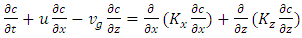 | (1) |
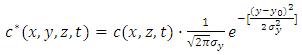 | (2) |
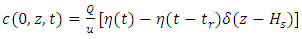 | (3) |
3. Results and Discussion
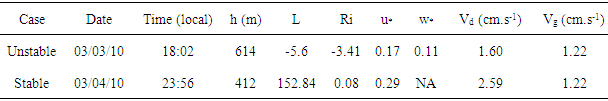
- The results of this work are shown on the following. Observed and calculated wind profiles are exhibited in Figure 1. It is noticeable that, in both cases, the model underestimates the windspeed. However, the simulated values express a statistical correlation of 80% for the stable case and 89% for the unstable one. Figure 2 displays the profiles for the eddy diffusivity coefficients, as calculated by the model. The values obtained, as well as their vertical distribution, are according to the expected, meaning that the turbulence is more intense and vertically distributed on the unstable PBL, while the stable PBL presents much lower values, which are maximum on the lower portion of it.
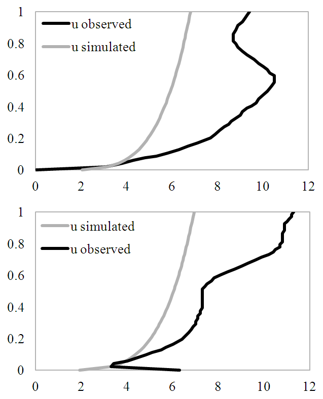 | Figure 1. Observed and simulated wind speed profiles (m.s-1) for the stable (top) and unstable (bottom) cases. Vertical axis displays the non-dimensional height (z/h) |
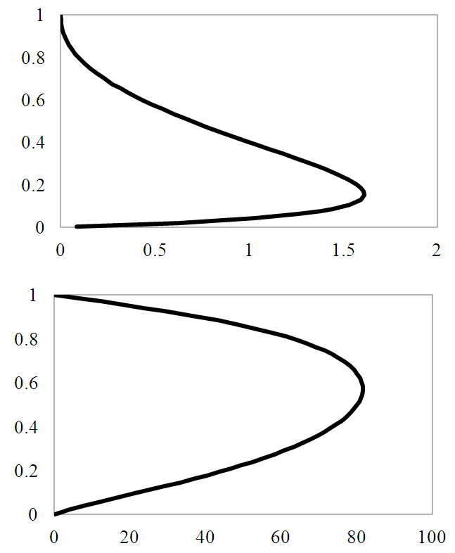 | Figure 2. Kz (m2.s-1) versus non-dimensional height for the stable (top) and unstable (bottom) cases |
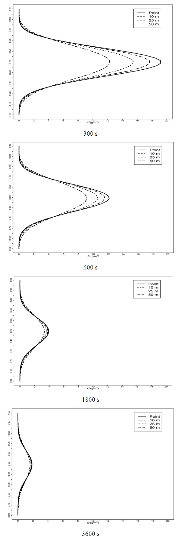 | Figure 3. Vertical profile of crosswind integrated concentration versus non-dimensional height for the stable case |
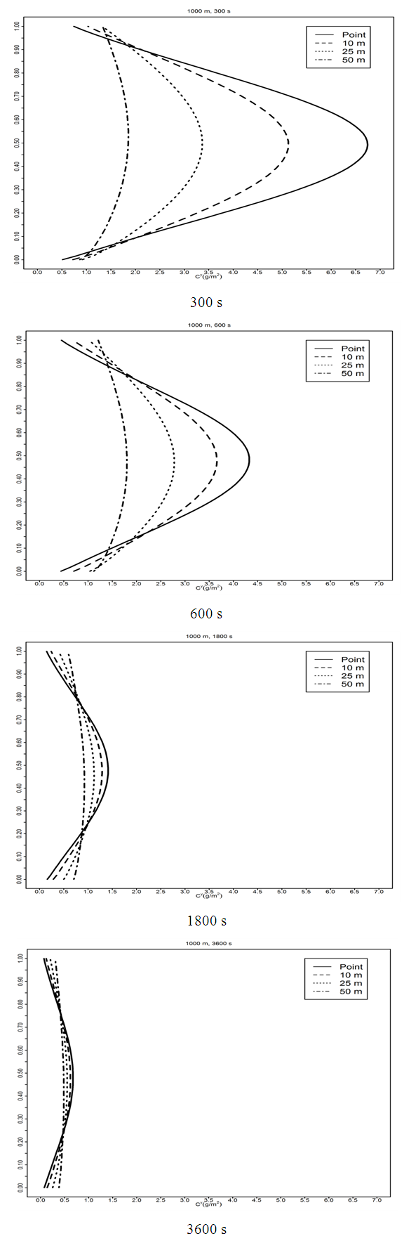 | Figure 4. Same as Figure 3, but for the unstable case |
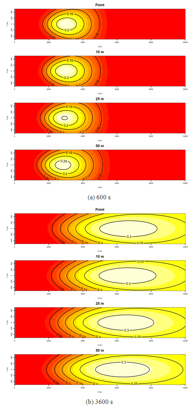 | Figure 5. Concentrations (mg.m-3) at z = 1 m for the stable case, and the different radiuses and instants |
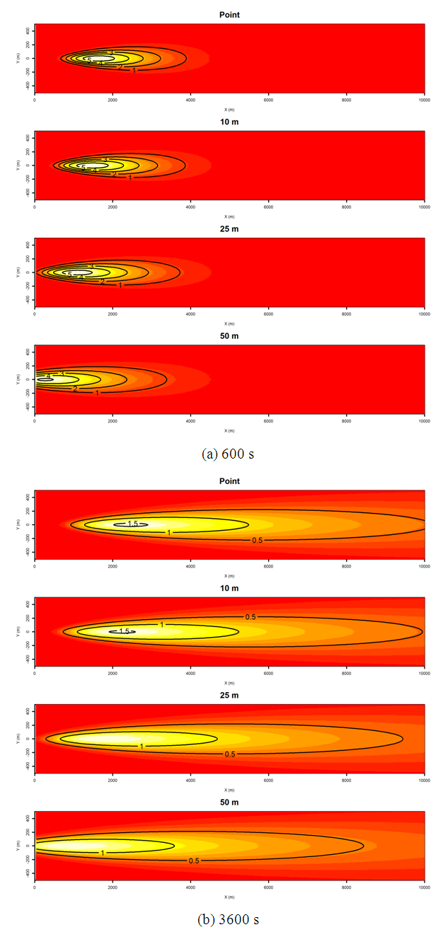 | Figure 6. Same as figure 5, but for the unstable case |
4. Conclusions and Remarks
- The results for the sensitivity tests regarding the volume of the emission source were shown, for the cases of a stable and unstable PBL. The model proved itself sensitive in such aspect, as well as presented differences related to the atmospheric stability regime. There are still improvements to be made in the model, in order to make it more realistic and able to reproduce, with more details, the phenomena inherent to the dispersion processes, especially in cases of rocket launching. However, it must be highlighted that, by using the GILTT, the computational cost of this analytical model is much lower than that of a numerical model, which allows its use in situations when there is need for quick results.
ACKNOWLEDGEMENTS
- The authors thank the Brazilian CNPq for funding the research.
References
| [1] | Nyman, R. L., NASA Report: “Evaluation of Taurus II Static Test Firing and Normal Launch Rocket Plume Emissions”, 2009. |
| [2] | Moreira, D. M.; Vilhena, M. T.; Buske, D.; Tirabassi, T., 2009, The state-of-art of the GILTT method to simulate pollutant dispersion in the atmosphere, Atmospheric Research, v. 92, p. 1-17. |
| [3] | Panofsky, H. A.; Dutton, J. A., 1984, Atmospheric Turbulence. John Wiley & Sons. New York, 387 p. |
| [4] | Degrazia, G. A.; Anfossi, D.; Carvalho, J. C.; Mangia, C.; Tirabassi, T.; Velho, H. F. C., 2000, Turbulence parameterisation for PBL dispersion models in all stability conditions. Atmospheric Environment, v. 34, p. 3575–3583. |
| [5] | Degrazia G. A., Rizza U, Mangia C, Tirabassi T, 1997, Validation of a new turbulent parameterization for dispersion models in a convective condition. Boudary Layer Meteorology, v. 85(2), p. 243-254, doi: 10.1023/A:1000474204748 |
| [6] | Bainy, B. K.; Buske, D.; Quadros, R. S., 2015, An analytic model for dispersion of rocket exhaust clouds: specifications and analysis in different atmospheric stability conditions, Journal of Aerospace Technology and Managagement, v. 7 (3), p. 374–385. |