Cibele A. Ladeia, Bardo E. J. Bodmann, Marco T. Vilhena
Department of Mechanical Engineering, University of Rio Grande do Sul, Porto Alegre, Brazil
Correspondence to: Cibele A. Ladeia, Department of Mechanical Engineering, University of Rio Grande do Sul, Porto Alegre, Brazil.
| Email: |  |
Copyright © 2018 The Author(s). Published by Scientific & Academic Publishing.
This work is licensed under the Creative Commons Attribution International License (CC BY).
http://creativecommons.org/licenses/by/4.0/

Abstract
In this work we present a solution for the radiative conductive transfer equation in cylinder geometry for a solid cylinder. We discuss a semi-analytical approach to the non-linear  problem, where the solution is constructed by Laplace transform and a decomposition method. The obtained solution allows then to construct the relevant near field to characterize the source term for dispersion problems when adjusting the model parameters such as albedo, emissivity, radiation conduction and others in comparison to the observation, that are relevant for far field dispersion processes and may be handled independently from the present problem. In addition to the solution method we also report some solutions and numerical simulations.
Keywords:
Radiative conductive transfer equation in cylinder geometry, Non-linear  problem, Decomposition method
Cite this paper: Cibele A. Ladeia, Bardo E. J. Bodmann, Marco T. Vilhena, The Radiative Conductive Transfer Equation in Cylinder Geometry: Rocket Launch Exhaust Phenomena for the Alcântara Launch Center, American Journal of Environmental Engineering, Vol. 8 No. 4, 2018, pp. 118-127. doi: 10.5923/j.ajee.20180804.06.
1. Introduction
During the last decades, aerospace engineering includes among others extensive research on the radiative conductive transfer equation [1, 2]. The problem pertinent involving this equation is rocket launch exhaust. To launch a rocket or to move a rocket through space, a propulsion system is needed to generate thrust. Thrust is produced by burning solid or liquid fuel, where hot combustion products are released into the atmosphere. In order to predict and control rocket launching, counties with such facilities make use of algorithms that analyze, before a launch, the trajectory of the gases [3]. So far, Brazil has no applicable model to meet this demand, so that a model for this purpose is being developed [4] and [5]. The Alcântara Launch Center is the Brazilian access to space, located in the northeastern region of Brazil. It is noteworthy that Alcântara has a privileged location among the locations used worldwide to launch space vehicles, due to its proximity to the equator. Despite the usefulness of investments in space activities, launches represent a considerable source of pollution despite being of singular character. It should be noted that codes exist that consider meteorological aspects and those of dispersion, which are usually valid far from the source and in addition super-simplify or discard thermal effects of the polluting source. The present work aims to progress in this aspect and to characterize the main thermal aspects of the source, addressing the near field by the radiative conductive transfer equation. In this context, this work obtains a solution for the equation of radiative conductive transfer in cylinder geometry. Solutions found in the literature are typically determined by numerical means, see, for instance [6, 7, 8]. Recently, the authors proved consistency and convergence of the solution obtain by decomposition method inspired by stability analysis criteria and taking into account the influence of the parameter sets [9]. The solution was constructed using Laplace transform together with a decomposition method [10]. The Laplace method is related to procedures for linear problems, while the decomposition method allows to treat the non-linear contribution as source term in a linear recursive scheme and thus opens a pathway to determine a solution, in principle to any prescribed precision [10].The present work is a continuation of [11], where the focus was put on the development of the formalism, deriving a solution and the computational algorithm. Differently than other works [6, 12, 7, 8], the radiative-convective problem was evaluated with the two angles treated individually, also manifest in the specific choice of the quadratures that approximate the scattering integral.In the present discussion, we will show the correlations between physical parameters, such as albedo, emissivity, radiation conduction among others, can be related to density or pollutant concentration profile in the exhaust gas in rocket launch. Furthermore, some of the numerical results are presented.
2. The Radiative Conductive Transfer Equation in Cylinder Geometry
We consider the one-dimensional steady state problem in cylindrical geometry for a solid cylinder. The problem of energy transfer is described in [13] by the radiative conductive transfer equation coupled to the energy equation, with 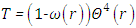 ,
, | (1) |
for  and
and  Here,
Here,  ,
,  is the polar angle,
  ,
,  is the azimuthal angle, I is the radiation intensity,
  is the single scattering albedo and
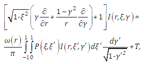
  signifies the differential scattering coefficient, also called the phase function [14]. In this work, we consider polar symmetry due to translational symmetry along the cylinder axis. Moreover, the isotropic medium implies azimuthal symmetry. The integral on the right-hand side of (1) can be written as
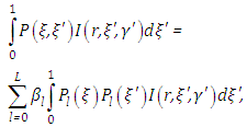 where
where  are the expansion coefficients of the Legendre polynomials
  and L refers to the degree of anisotropy, for details see [10]. The energy equation for the temperature that connects the radiative flux to a temperature gradient is
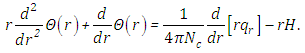 | (2) |
Here,  is the radiation conduction parameter with
  the thermal conductivity,
  the extinction coefficient, the Stefan-Boltzmann constant,
  the refractive index,
  is a reference temperature,
 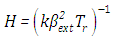 is a normalised π constant, and
  is used to denote a prescribed heat generation in the medium that is independent of the radiation intensity. The dimensionless radiative heat flux is expressed in terms of the radiative intensity by
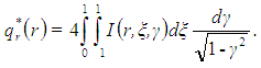 For diffuse emission and diffuse reflection the boundary conditions of equation (1) are
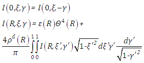 for
for  and
and  is the diffuse reflectivity,
  is the emissivity, the thermal photon emission according to the Stefan-Boltzmann law (see [15]). In the equation (2), we notice that
  is not a physical boundary, and for solution
  to be physically meaningful we need to impose at
  the implicit boundary condition, i.e., the solution remains bounded at the origin. The boundary condition of equation (2) is
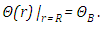 | (3) |
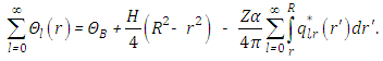
In addition, if the radiative heat flux is known, we can solve (2) and use equation (3) to find | (4) |
3. Solution by the Decomposition Method
In order to obtain a solution, we use the  approximation extended by an additional angular variable
 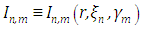 . The
. The  approximation [14], is based on the angular variable discretisation of
  in an enumerable set of angles or equivalently their direction cosines, in our work
  and
and  . Then the equations (1) and (2) can be simplified using an enumerable set of angles following the collocation method, which defines the problem of radiative conductive transfer in cylindrical geometry in the so-called
  approximation,
 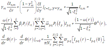 | (5) |
Here n indicates a discrete direction of  and m a discrete direction of
  , respectively. The
  are the weights from the quadratures that approximate the integrals explained in detail further down. The integration is carried out over two octants with
  and
and  . In this approximation equation (5) may be written as
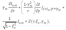 | (6) |
where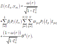 Instead of
 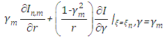 , we take as independent variables
  and
and 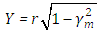 , for
, for  and
and  . Then equation (6) becomes
 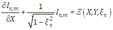 or in
or in  representation
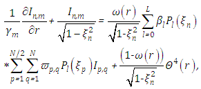 | (7) |
 | (8) |
Here  and
and  are evaluation points, with
  and
and  and subject to the following boundary conditions:
  As already indicated above, the integrals over the angular variables are replaced by Gauss-Legendre and Gauss-Chebyshev quadratures with weight
  , with Gauss-Legendre weight normalisation
  and Gauss-Chebyshev weight normalisation to the solid angle of an octant
 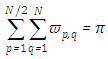 . The choice for the specific quadratures is due to the phase function representation in terms of Legendre polynomials, and the second quadrature scheme by the singular structure of the integral, that is found in representations for Chebyshev polynomials. The equations system (7) and (8) may be cast in a first order differential equation system in matrix form
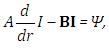 | (9) |
where  is a diagonal matrix of order
  , with
  ,
,  is a square matrix of the same order as
  with elements
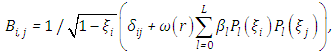
 is the usual Kronecker symbol and the vector of the intensity of order
  is defined by
 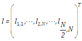 . The non-linear terms are
  sequences of
  identical angular terms for the
  directions.
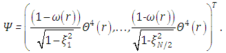 According to [10] the intensity of radiation is expanded in an infinite series
  , thus introducing an infinite number of artificial degrees of freedom which may be used to set up a non-unique recursive scheme of linear differential equations, where the non-linear terms appear as source term containing known solutions
  from the previous recursion steps [10] and the solution of the linear differential equations is known. Equation (9) is then
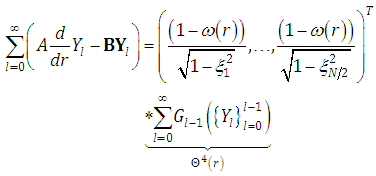 | (10) |
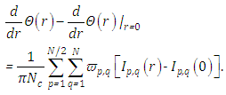
In order to solve the equation system (10) in a recursive fashion, the initialisation is chosen to be  further subject to the original boundary conditions and then making use of a recursive process of the equations for the remaining components
  with homogeneous boundary conditions.
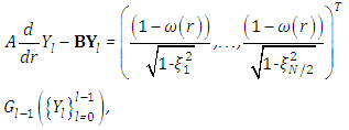 | (11) |
with  . Accordingly the recursion initialisation corresponds to the homogeneous solution where all subsequent recursion steps result in particular solutions. The remaining,
  denotes the inverse Laplace transform operator, s is the r dual complex variable from Laplace transform of equation (11),
  and the decomposed matrix
  with
with  the diagonal matrix with distinct eigenvalues and
  the eigenvector matrix.
 | (12) |
The general solution for each decomposition term  is explicitly given by
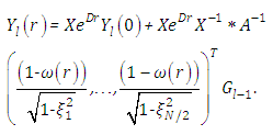 The non-linearity from the temperature term
 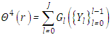 is represented by Adomian polynomials
  . In the following the notation
  stands for the
  functional derivative of the non-linearity at
  , so that one may identify the first term
  and all the subsequent terms of the series that define the Adomian polynomials
  as shown below (for details see [10]).
 | (13) |
Here  are the usual multinomial coefficients. In principle one has to solve an infinite number of equations, so that in a computational implementation one has to truncate the scheme according to a prescribed precision. Recently, the authors proved consistency and convergence of the solution obtained by decomposition method inspired by stability analysis criteria and taking into account the influence of the parameter sets [9]. From the last term in equation (13) one observes that for a non-linearity with polynomial structure there is only a limited number of combinations in the last term. Consequently, for j sufficiently large the factorial term
  controls the magnitude of the correction terms, which for increasing j tend to zero. One may now determine the temperature profile. To this end and in order to stabilize convergence a correction parameter
  for the recursive scheme was introduced, where
  , with
  ,
, | (14) |
A remark on the use of the correction parameter  is in order here. For some of the parameter combinations the solution did not converge. In order to stabilize convergence where necessary,
  was changed in a decrement succession from 10 to 0.1 which corresponds to weak (for
  ) up to strong (for
  ) corrections until stable results were obtained. More specifically, the stabilization of convergence was implemented as follows. Due to the non-uniqueness of the recursive scheme the non-linearity is split and distributed in various recursion steps instead of considering the full non-linearity in one step, thus delaying the inclusion of the non-linearity in the solution. It is noteworthy, that this procedure does not change the physical model but only its mathematical representation. Consequently, for large
  a smaller number of recursions absorb the decomposed non-linearity whereas for small
  the non-linearity is distributed in a larger number of recursion steps.
4. Numerical Results and Discussions
Below, we implement a fictitious scenario, exhaust plume, to test consistency of the proposed method. For simplicity, the exhaust plume is assumed to have uniform temperature and constant properties, not dependent on space and wavelength. To this end we determine characteristic quantities for the radiative conductive transfer problem, which are the profiles of the normalized temperature, the radiative, conductive and total heat fluxes, respectively.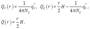 | (15) |
All the numerical results are based on the seven cases specified below, we consider isotropic scattering  in units of
  that varies between 0 and 1. In this analysis,
  directions were used (note that
  is the discrete direction of the polar variable and
  is the discrete direction of the azimuthal variable, hence the order of the quadrature is equal to 8). As a first step in evaluating our solution, we solved cases 1-6 we consider
  , i.e. without heat generation in the medium. In this cases 7 we investigate the influence of parameter
  Furthermore, the cases 1-3 we investigate the influence of parameter
  , and the cases 4-6 we investigate the influence of parameter
  . These parameters, such as
  and
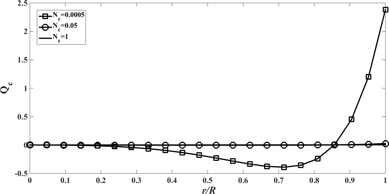
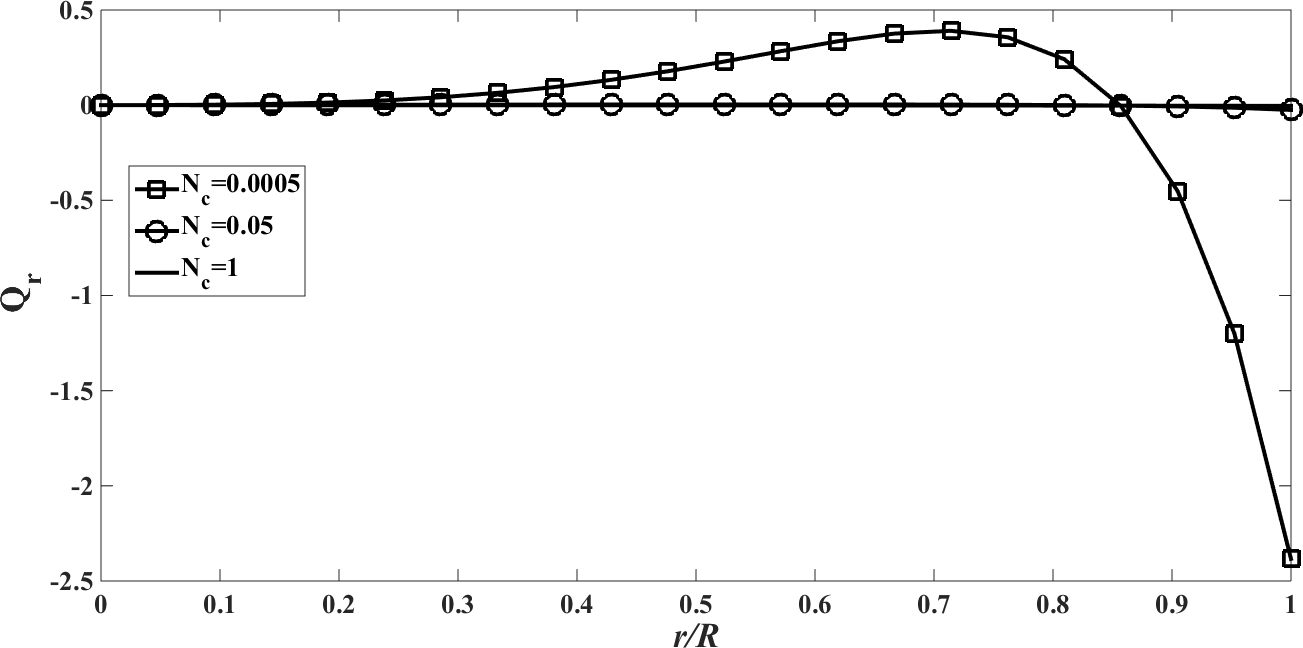
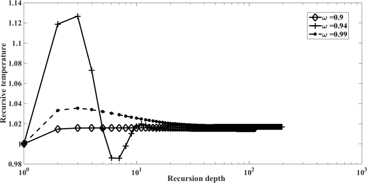
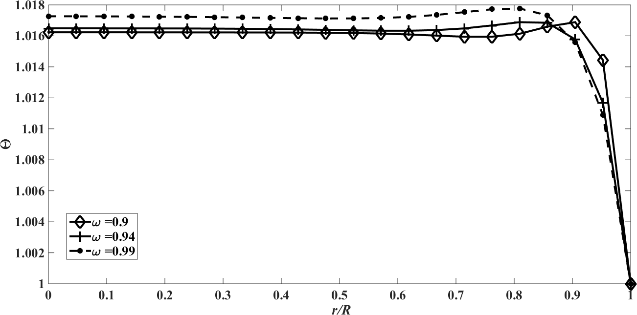
and  , can be reported in the concentration of pollutant in the exhaust that allows to model the near field, the source term for pollutant dispersion during rocket launch.In the Figures, the abscissa represents the number of recursions that attain a specified precision henceforth denoted as recursion depth.Case 1. In this case, the results are based on the parameter set with
  and
and  . The numerical results for the profile of the temperature
  , the conductive heat flux
  and the radiative heat flux
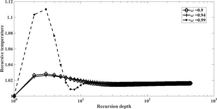
  and the temperature after a number of recursion steps are shown Figures. 1, 2, 3 and 4, respectively, where we consider
  . We used as a stopping criterion the last twenty recursions of temperature changing less than,
  , so that, the series of Adomian polynomials was truncated at
  for
for  ,
,  for
for  and
and  for
for  .
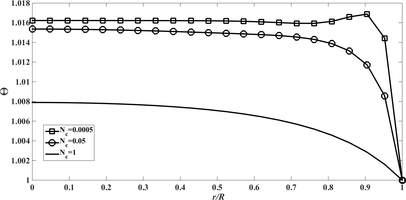
. | Figure 1. The temperature profile  against the relative optical depth, (case 1) against the relative optical depth, (case 1) |
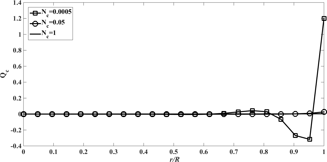
 | Figure 2. The conductive heat flux  against the relative optical depth, (case 1) against the relative optical depth, (case 1) |
 | Figure 3. The radiative heat flux  against the relative optical depth, (case 1) against the relative optical depth, (case 1) |
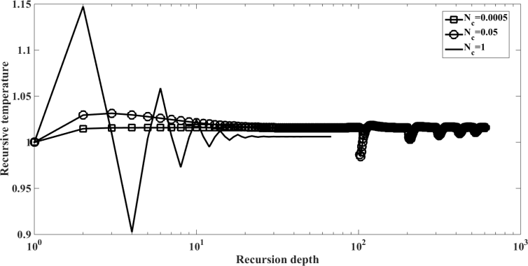
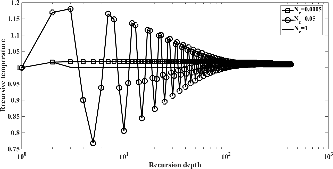 | Figure 4. Recursion temperature at  against recursion depth, (case 1) against recursion depth, (case 1) |
Case 2. In this case, the results are based on the parameter set with  and
and  . The numerical results for the profile of the temperature
  the conductive heat flux
  and the radiative heat flux
  and the temperature after a number of recursion steps are shown Figures. 5, 6, 7 and 8, respectively, where we consider
  . We used as a stopping criterion the last twenty recursions of temperature changing less than,
  , so that, the series of Adomian polynomials was truncated at
  for
for  ,
,  for
for  and
and  for
for  .
. | Figure 5. The temperature profile  against the relative optical depth, (case 2) against the relative optical depth, (case 2) |
 | Figure 6. The conductive heat flux  against the relative optical depth, (case 2) against the relative optical depth, (case 2) |
 | Figure 7. The radiative heat flux  against the relative optical depth, (case 2) against the relative optical depth, (case 2) |
 | Figure 8. Recursion temperature at  against recursion depth, (case 2) against recursion depth, (case 2) |
Case 3. In this case, the results are based on the parameter set with  and
and  . The numerical results for the profile of the temperature
  the conductive heat flux
  and the radiative heat flux
  and the temperature after a number of recursion steps are shown Figures. 9, 10, 11 and 12, respectively, where we consider
  . Again, the stopping criterion was chosen such that the last twenty recursions of temperature changed less than,
  . Here, the series of Adomian polynomials was truncated at
  for
for  for
for  and
and  for
for  .
. | Figure 9. The temperature profile  against the relative optical depth, (case 3) against the relative optical depth, (case 3) |
 | Figure 10. The conductive heat flux  against the relative optical depth, (case 3) against the relative optical depth, (case 3) |
 | Figure 11. The radiative heat flux  against the relative optical depth, (case 3) against the relative optical depth, (case 3) |
 | Figure 12. Recursion temperature at  against recursion depth, (case 3) against recursion depth, (case 3) |
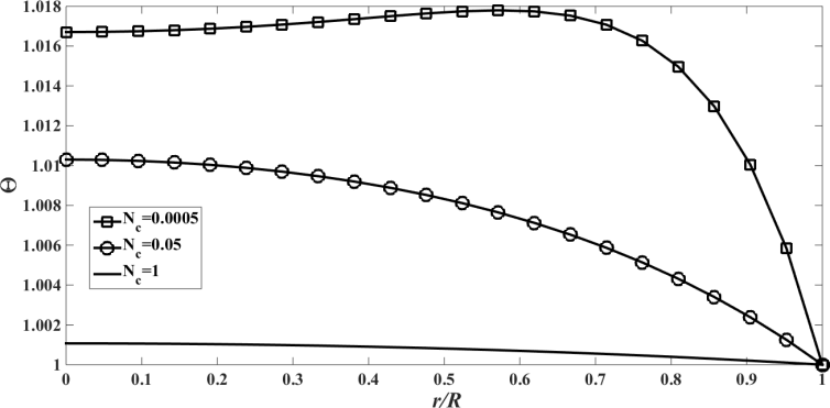
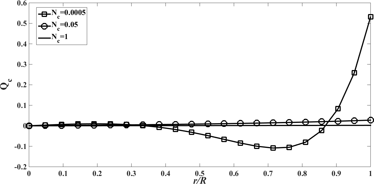
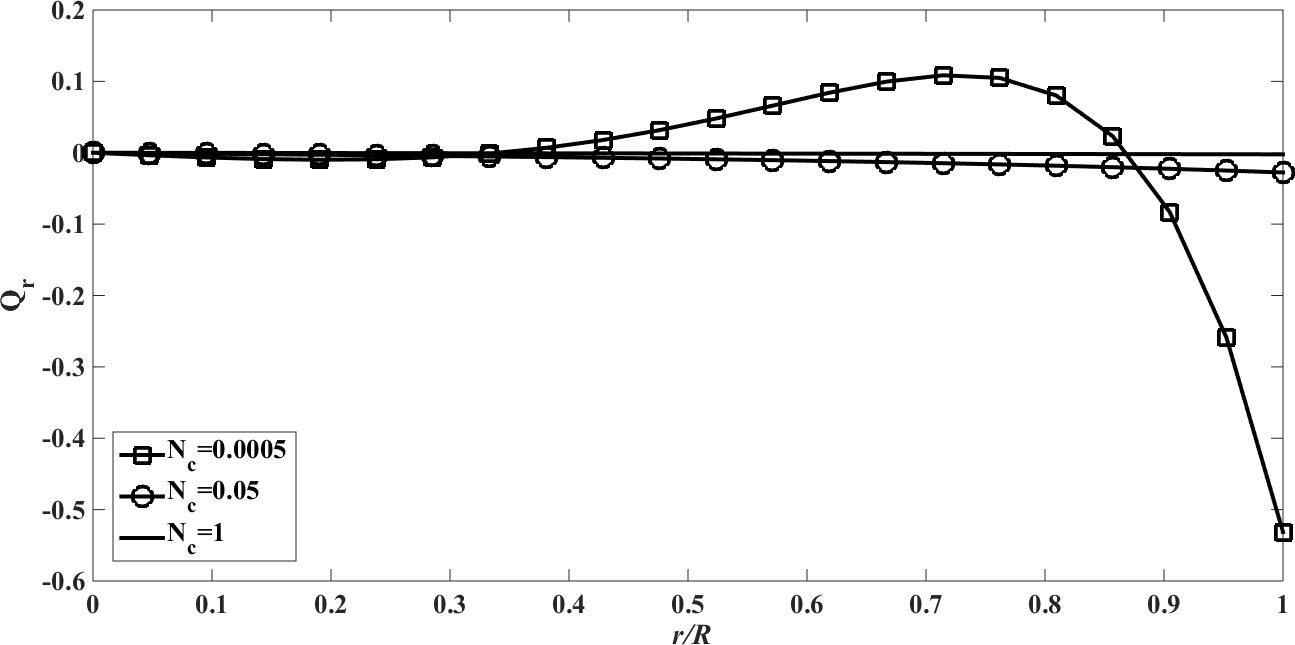
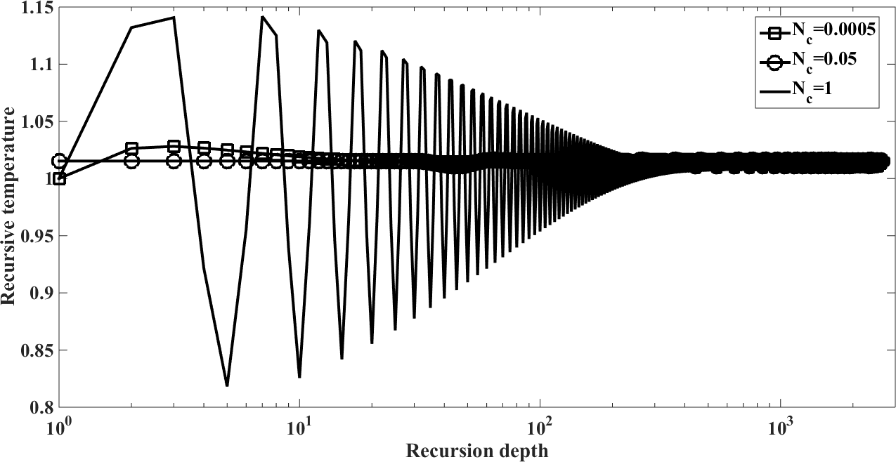
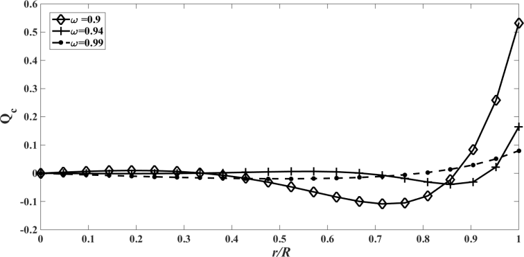
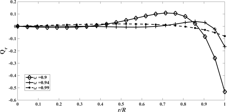
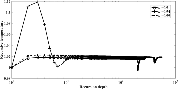
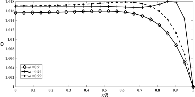
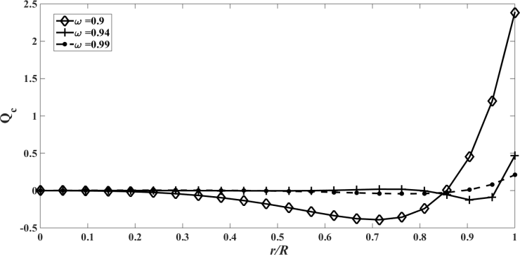
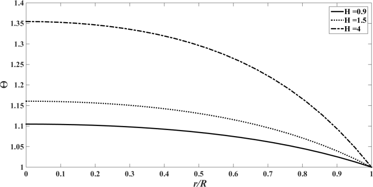
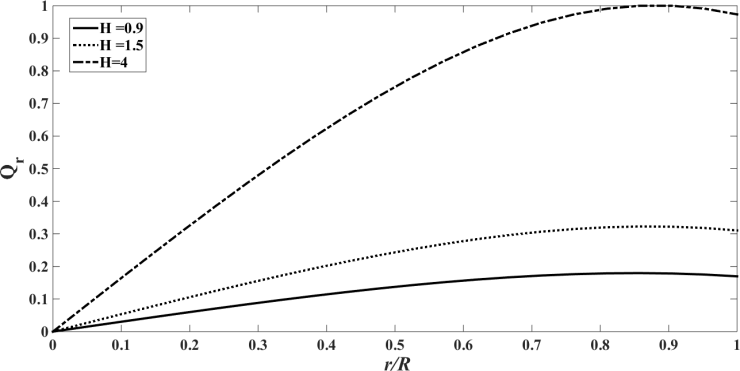
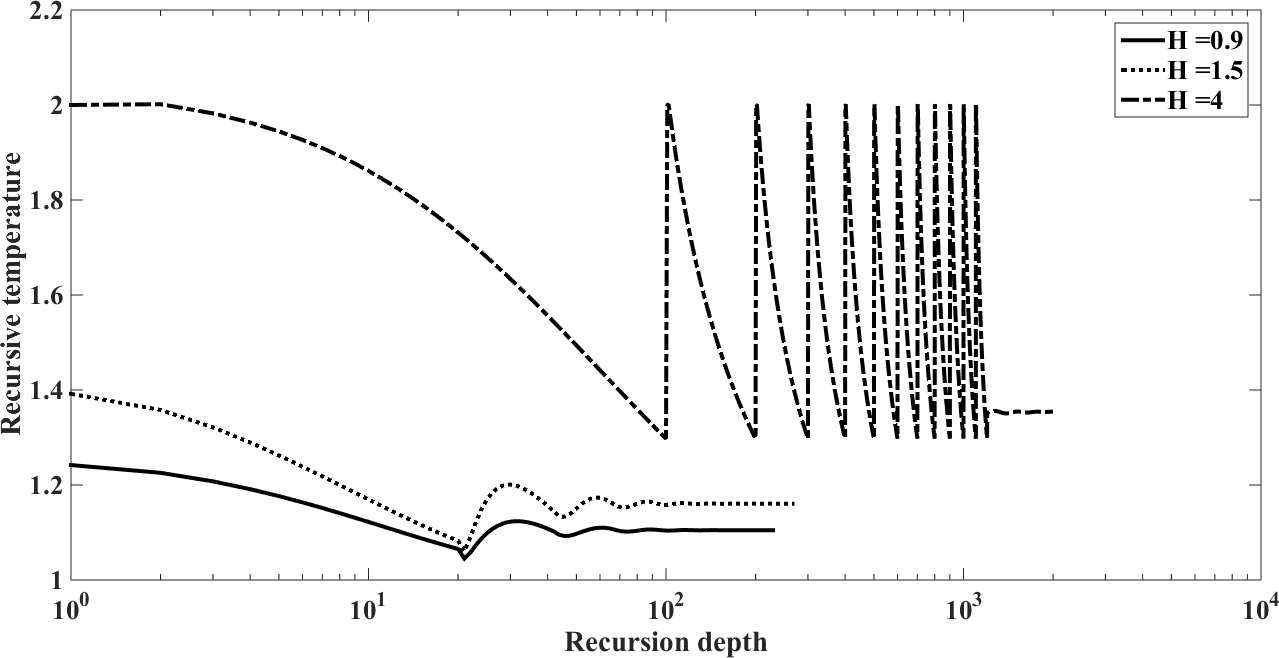
In the Figures. 1 - 12 are illustrated the effect of the radiation conduction parameter,  ; 0.05 and 1. According to the Figures. 1, 5 and 9 we note that for large value of
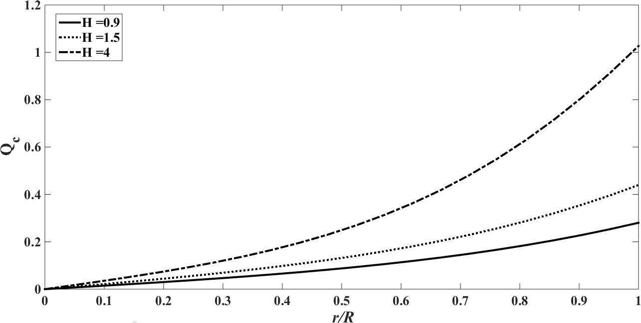
  , corresponds to the conduction-dominating case, the temperature profile is almost linear, while for the small value, radiation-dominating case, the temperature distribution is variable. In addition, note that the conductive heat fluxes (Figures. 2, 6 and 10), passes through the minimum point and the radiative heat fluxes (Figures. 3, 7 and 11), has corresponding maximum point whereas total heat fluxes, satisfies equation (15).Case 4. In this case, the results are based on the parameter set with
  and
and  . The numerical results for the profile of the temperature
  the conductive heat flux
  and the radiative heat flux
  and the temperature after a number of recursion steps are shown Figures. 13, 14, 15 and 16, respectively, where we consider
  . We used the same stopping criterion as for the previous cases. Accordingly, the series of Adomian polynomials was truncated at
  for
for  for
for  and
and  for
for 
 | Figure 13. The temperature profile  against the relative optical depth, (case 4) against the relative optical depth, (case 4) |
 | Figure 14. The conductive heat flux  against the relative optical depth, (case 4) against the relative optical depth, (case 4) |
 | Figure 15. The radiative heat flux  against the relative optical depth, (case 4) against the relative optical depth, (case 4) |
 | Figure 16. Recursion temperature at  against recursion depth, (case 4) against recursion depth, (case 4) |
Case 5. In this case, the results are based on the parameter set with  and
and  . The numerical results for the profile of the temperature
  the conductive heat flux
  and the radiative heat flux
  and the temperature after a number of recursion steps are shown Figures. 17, 18, 19 and 20, respectively, where we consider
  . We used the stopping criterion from the previous cases. Here, the series of Adomian polynomials was truncated at
  for
for 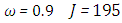 for
for  and
and  for
for  .
. | Figure 17. The temperature profile  against the relative optical depth, (case 5) against the relative optical depth, (case 5) |
 | Figure 18. The conductive heat flux  against the relative optical depth, (case 5) against the relative optical depth, (case 5) |
 | Figure 19. The radiative heat flux  against the relative optical depth, (case 5) against the relative optical depth, (case 5) |
 | Figure 20. Recursion temperature at  against recursion depth, (case 5) against recursion depth, (case 5) |
Case 6. In this case, the results are based on the parameter set with  and
and  . The numerical results for the profile of the temperature
  the conductive heat flux
  and the radiative heat flux
  and the temperature after a number of recursion steps are shown Figures. 21, 22, 23 and 24, respectively, where we consider
  . Here the stopping criterion with temperature change less than,
  was satisfied after
  for
for  for
for  and
and  for
for  .
. | Figure 21. The temperature profile  against the relative optical depth, (case 6) against the relative optical depth, (case 6) |
 | Figure 22. The conductive heat flux  against the relative optical depth, (case 6) against the relative optical depth, (case 6) |
 | Figure 23. The radiative heat flux  against the relative optical depth, (case 6). against the relative optical depth, (case 6). |
 | Figure 24. Recursion temperature at  against recursion depth, (case 6) against recursion depth, (case 6) |
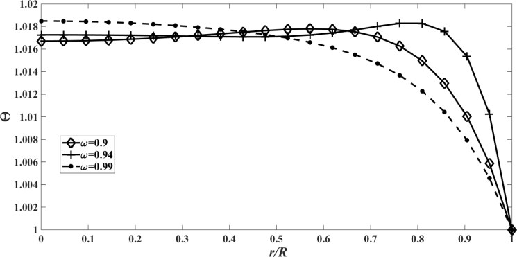
In the Figures. 13 - 24 are illustrated the effect of the albedo,  and
and  . For these cases the radiation conduction parameter was fixed at
  , that characterizes a situation in which energy transport by radiation is dominant, in this situation the effect of albedo is more significant. Note that
  is purely scattering medium and as a consequence can be seen by equations (1) and (2), that the temperature becomes independent of the radiative process and results in a linear profile. Similar to the previous case, the conductive heat fluxes, (Figure. 14, 18 and 22), passes through the minimum point and the radiative heat fluxes, (Figure. 15, 19 and 23), has a corresponding maximum point and the total heat fluxes, satisfies equation (15), as expected.Case 7. In this case, the results are based on the parameter set with
  . The numerical results for the profile of the temperature
  the conductive heat flux
  and the radiative heat flux
  and the temperature after a number of recursion steps are shown Figures. 25, 26, 27 and 28, respectively, where we consider
  . We used the stopping criterion from the previous cases. Here, the series of Adomian polynomials was truncated at
  for
for  for
for  and
and  for
for  .
. | Figure 25. The temperature profile  against the relative optical depth, (case 7) against the relative optical depth, (case 7) |
 | Figure 26. The conductive heat flux  against the relative optical depth, (case 7) against the relative optical depth, (case 7) |
 | Figure 27. The radiative heat flux  against the relative optical depth, (case 7) against the relative optical depth, (case 7) |
 | Figure 28. Recursion temperature at  against recursion depth, (case 7) against recursion depth, (case 7) |
The results in Figures. 25 - 28 show the influence of  and 4, that is, constant generation of heat that is independent of the intensity of radiation. Note that as
  increases, the temperature also increases, which is to be expected since more energy enters into the system. The values of
  were chosen aiming at the order of magnitude, since there is a lack of data in the literature to estimate this parameter.The values of the
  are related to the contributions to correction of the recursive scheme. These values range from 10 to 0.1, where 10 and 1 are minor contributions to correction, while 0.1 are major contributions to correction. In addition, we can observe in Figures. 4, 8, 12, 16, 20, 24 and 28 in order to obtain numerical stability many Adomian terms are required. However, there is also the influence of the other parameters such as
  emissivity and
  diffuse reflectivity. The emissivity and diffuse reflectivity are related to the boundary conditions of the radiation intensity.
5. Conclusions
In the present work we presented a semi-analytical solution for the radiative conductive transfer equation in cylinder geometry and in  approximation. The authors consider the developments as one step into a direction where the solutions may be used to characterize the near field, i.e. a hot source of a pollution dispersion problem, more specifically the release of hot substances due to rocket launch. These conditions model the initial condition for the dispersion problem, that generates the pollution concentrations of the far field. To this end the original non-linear radiative-conductive transfer problem was decomposed in a recursive scheme of equation systems by the use of a modified decomposition method, following the reasoning of references [10, 11]. The initialization of the recursion is a linear equation system with known solution and subject to the original boundary conditions. All the subsequent equation systems to be solved are of linear type, where the non-linearity appears as source term that contains only terms from solutions of all previous recursion steps. It is noteworthy that the recursive scheme is not unique and convergence depends strongly on the recursion initialization.From the physical point of view, a set of parameters was chosen for the which the law of conservation of energy was as expected. In addition, a correction parameter was considered for the recursive scheme since without this correction the scheme fails to converge due to arithmetic imprecisions and instabilities. As a result of this work we showed a relation between the physical parameters, albedo, emissivity, radiation conduction among others, which may be related to the density or concentration of pollutants in the exhaust gases emitted in a rocket launch. Such a relationship is essential because dispersion models of existing pollutants are characterized by the absence of thermal properties of the source, so that an extension of the present study in this direction may open pathways to introduce these features into simulations. As future work, we intend to further investigate which physical parameters are in fact adequate for the problem in question.
ACKNOWLEDGEMENTS
The authors thank CAPES and CNPq for financial support.
References
| [1] | M. F. Modest, Radiative Heat Transfer, New York, McGraw-Hill, 1993. |
| [2] | J. R. Howell, M. P. Menguc, R. Siegel, Thermal Radiation Heat Transfer, CRC Press, New York, 2016. |
| [3] | J. R. Bjorklund, J. K. Dumbauld, C. S. Cheney, H. V. Geary, User's Manual for the REEDM (Rocket Exhaust Effluent Diffusion Model) Computer Program, NASA contractor report 3646. NASA George C. Marshall Space Flight Center, Huntsville, AL, 1982. |
| [4] | D. M. Moreira, L. B. Trindade, G. Fisch, M. R. Moraes, R. M. Dorado, R. L. Guedes, A multilayer model to simulate rocket exhaust clouds, Journal of Aerospace Technology and Management 3 (2011), 41-52. |
| [5] | D. Schuch, G. Fisch, The use of an atmospheric model to simulate the rocket effluents transport dispersion for the centro de lançamento de Alcântara, Journal of Aerospace Technology and Management 9 (2017), 137-146. |
| [6] | H. Li, M. Ozisik, Simultaneous conduction and radiation in a two-dimensional participating cylinder with anisotropic scattering, Journal of Quantitative Spectroscopy and Radiative Transfer 46 (1991), 393-404. |
| [7] | H.-Y. Li, A two-dimensional cylindrical inverse source problem in radiative transfer, Journal of Quantitative Spectroscopy and Radiative Transfer, 60 (2001), 403-414. |
| [8] | S. C. Mishra, C. H. Krishna, M. Y. Kim, Analysis of conduction and radiation heat transfer in a 2-d cylindrical medium using the modified discrete ordinate method and the lattice boltzmann method, Numerical Heat Transfer 60 (2011), 254-287. |
| [9] | C. A. Ladeia, B. E. J. Bodmann, M. T. Vilhena, The radiative conductive transfer equation in cylinder geometry: Semi-analytical solution and a point analysis of convergence, Journal of Quantitative Spectroscopy and Radiative Transfer 217 (2018), 338-352. |
| [10] | M. T. M. B. Vilhena, B. E. J. Bodmann, C. F. Segatto, Non-linear radiative-conductive heat transfer in a heterogeneous gray plane-parallel participating medium, In: Ahsan, A. (ed.) Convection and Conduction Heat Transfer. InTech (2011), 177-196. |
| [11] | C. A. Ladeia, B. E. J. Bodmann, M. T. B. Vilhena, The radiative-conductive transfer equation in cylinder geometry and its application to rocket launch exhaust phenomena, Integral Methods in Science and Engineering (2015), 341-351. |
| [12] | C. E. Siewert, J. R. Thomas Jr., On coupled conductive-radiative heat transfer problems in a cylinder, Journal of Quantitative Spectroscopy and Radiative Transfer 48 (1992), 227-236. |
| [13] | M. Ozisik, Radiative transfer and interactions with conduction and convection, John Wiley & Sons Inc., New York, 1973. |
| [14] | S. Chandrasekhar, Radiative Transfer, Oxford University Press, New York, 1950. |
| [15] | A. Elghazaly, Conductive-radiative heat transfer in a scattering médium with angle-dependent reective boundaries, Journal of Nuclear and Radiation Physics 4 (2009), 31-41. |

 Abstract
 Reference
 Full-Text PDF
 Full-text HTML