-
Paper Information
- Next Paper
- Previous Paper
- Paper Submission
-
Journal Information
- About This Journal
- Editorial Board
- Current Issue
- Archive
- Author Guidelines
- Contact Us
American Journal of Environmental Engineering
p-ISSN: 2166-4633 e-ISSN: 2166-465X
2018; 8(4): 112-117
doi:10.5923/j.ajee.20180804.05

On a Model for Pollutant Dispersion in the Atmosphere with Partially Reflective Boundary Conditions and Data Simulation Using CALPUFF
 Abstract
 Reference
 Full-Text PDF
 Full-text HTML
Jaqueline Fischer Loeck1, Juliana Schramm1, Bardo Bodmann2
1Graduate Program in Mechanical Engineering, Federal University of Rio Grande do Sul, Porto Alegre, Brazil
2Federal University of Rio Grande do Sul, Porto Alegre, Brazil
Correspondence to: Jaqueline Fischer Loeck, Graduate Program in Mechanical Engineering, Federal University of Rio Grande do Sul, Porto Alegre, Brazil.
| Email: |  |
Copyright © 2018 The Author(s). Published by Scientific & Academic Publishing.
This work is licensed under the Creative Commons Attribution International License (CC BY).
http://creativecommons.org/licenses/by/4.0/

The present work is an attempt to simulate the dispersion of pollutants in the surroundings of the thermoelectric plant located in Linhares from a new mathematical model based on partially reflective boundaries in the deterministic advection-diffusion equation. In addition to the advection-diffusion equation with partially reflective boundaries, it was used data simulated with the CALPUFF model. The exposed model was validated previously with the Hanford and Copenhagen experiments and the results indicate that effects on the boundaries are essential to model dispersion phenomenona in the atmospheric boundary layer.
Keywords: Advection-diffusion equation, Reflective boundary conditions, CALPUFF
Cite this paper: Jaqueline Fischer Loeck, Juliana Schramm, Bardo Bodmann, On a Model for Pollutant Dispersion in the Atmosphere with Partially Reflective Boundary Conditions and Data Simulation Using CALPUFF, American Journal of Environmental Engineering, Vol. 8 No. 4, 2018, pp. 112-117. doi: 10.5923/j.ajee.20180804.05.
Article Outline
1. Introduction
- The development of mathematical models is fundamental for environmental management once it can calculate the whole concentration field of pollutants based on the local micrometeorological data. Over the years there has been an improvement not only in technology, but also in mathematical techniques whether numerical or analytical, which makes the models closer to the phenomenon they are mimicking. Although the dispersion of pollutants phenomenon is not deterministic, its modelling usually is, that means there will always be a difference between simulation and measurements. As an attempt to diminish this difference between simulation and measurements, the well-known advection-diffusion equation is solved making use of modified boundary conditions. In a previous work [11] this model was validated with reference experiments such as Hanford [8] and Copenhagen [9] and in the sense of high agreement between data and model, the results were significant. For this reason, the present work has the objective of using the presented model, together with simulated data from the model CALPUFF, to obtain the concentration field of pollutants in the surroundings of the thermoelectric plant located in Linhares – ES, Brazil.
2. A Locally Gaussian Model
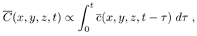
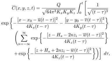
- The advection-diffusion equation can be obtained from the continuity equation making use of Reynolds decomposition to separate the mean components for the concentration and the velocity fields. Upon taking averages and substitution of the average fluctuations by Fick's closure, where it is assumed that the turbulent flow of concentration is proportional to the magnitude of the mean concentration gradient, the desired equation for mean concentrations is attained. Considering the source term as an instantaneous initial condition denoted by the Dirac delta functions, and the diffusive coefficients Kx, Ky and Kz (m²/s) locally constant, the initial value problem that models the dispersion of a puff is given by [1, 16]
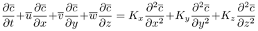 | (1) |
 | (2) |
 | (3) |
 | (4) |
3. Reflective Boundary Conditions
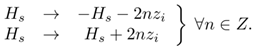
- To justify the mapping of the infinite range z ∈ (−∞, ∞) to the finite z ∈ [0, zi] we first consider a cut of the distribution at z=0 and z=zi, respectively. Formally, the reflection on the ground and in the atmospheric boundary layer may be viewed as contributions due to a virtual source in some effective heights to both sides below ground and above the boundary layer [2], those heights are the center of the gaussians formed at the ground and at the top of the atmospheric boundary layer. The sequences that represent the mirror maxima are
 | (5) |
 | (6) |
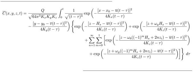 | (7) |
4. Turbulent Diffusivity Parametrisation
- The parametrisation for the eddy diffusion coefficient for convective conditions is based on the turbulent diffusion theory [18] and on the turbulent kinetic energy spectrum [14] and is given by [6]
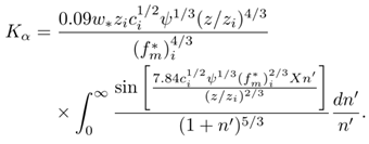 | (8) |
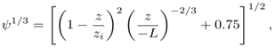 | (9) |
4.1. Wind Speed Profile
- The wind speed profile was parametrised according to the Monin-Obukhov's similarity theory and the OML-model [3], where close to the surface and because of its roughness, there is a raising profile, whereas sufficiently far from the surface the wind speed remains approximately constant. If zb = min(|L|, 0.1zi), then
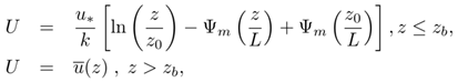 | (10) |
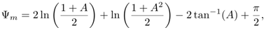 | (11) |
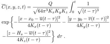
5. Methodology
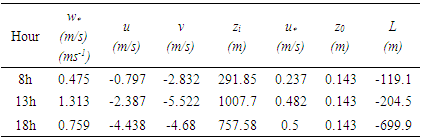
- The thermoelectric plant that was simulated consists of 24 continuous emission chimneys, and for this purpose each of the chimneys was simulated by the solution (7). Subsequently, the solution for each of the chimneys was superimposed. In addition to the source data, it was used the CALPUFF model in the version of the system officially approved by the USEPA (United States Environmental Protection Agency) [19]. CALPUFF is a Gaussian non-stationary state puff type model that simulates pollutant packages that are transported and dispersed in a tridimensional field. The simulation makes use of the preprocessors TERREL, CTGPROC, MAKEGEO, SMERGE and READ62 for later use in the CALMET meteorological model. From the simulation it was obtained the data which its mean values are presented at Table 1, it was simulated for 1 hour of emission in three different hours, 8, 13 and 18 o'clock, with the intention to observe the variation of results throughout the day. In a first approach it was used averages of the data in the whole terrain, and then different values were used at each point of the terrain. The total distance simulated was 14 km in each direction.
|
6. Results
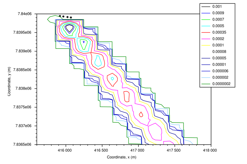
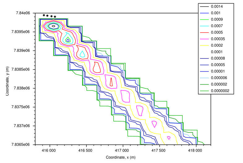
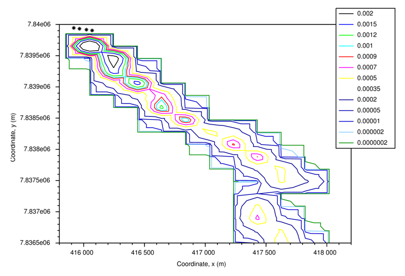
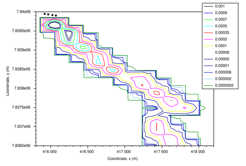
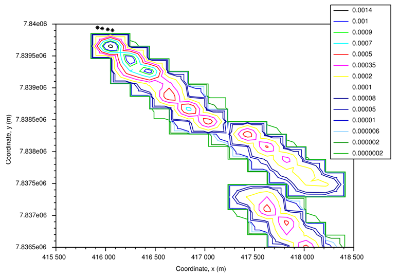
- In this section are presented the results of the simulations, it will be exposed the concentration contour lines (g/m³) for the 8, 13 and 18 o'clock simulations, respectively. Figures 1, 2 and 3 refer to the simulations using mean values of the data, exposed in Table 1. In Figures 4, 5 and 6 it was used different values of the data at each point of the terrain. All simulations presented make use of the reflection parameters ωb=ωg=0.3. Each asterisk (∗) refers to a group of 6 sources.
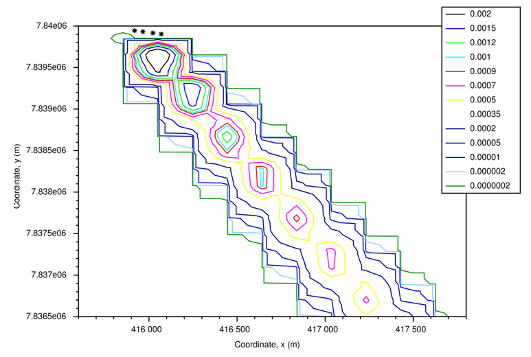 | Figure 1. Concentration contour lines (g/m³) for the simulation at 8 o'clock, using averages of the CALPUFF simulated data |
 | Figure 2. Concentration contour lines (g/m³) for the simulation at 13 o'clock, using averages of the CALPUFF simulated data |
 | Figure 3. Concentration contour lines (g/m³) for the simulation at 18 o'clock, using averages of the CALPUFF simulated data |
 | Figure 4. Concentration contour lines (g/m³) for the simulation at 8 o'clock, using the CALPUFF simulated data |
 | Figure 5. Concentration contour lines (g/m³) for the simulation at 13 o'clock, using the CALPUFF simulated data |
 | Figure 6. Concentration contour lines (g/m³) for the simulation at 18 o'clock, using the CALPUFF simulated data |
7. Conclusions
- The purpose of this work was to make use of data from CALPUFF together with a new mathematical model for pollutant dispersion and simulate the surroundings of a thermoelectric power located in Linhares - ES, Brazil. At first, only mean values of the data simulated by the CALPUFF model were used. Besides these data are not the best approximation, since the model is outdated, the use of averages also hinders proper simulation. When it was used different data for each point of the terrain, the concentration of pollutants has become more precise, despite the difficulty found in the simulated data, which contained errors. As future work, it is expected to obtain data from the meteorological tower settled on the site of the thermoelectric plant and then simulate the model without needing the data provided by CALPUFF, due to the problems found in them.
ACKNOWLEDGEMENTS
- This work was supported by Linhares Geração SA, Coordination for the Improvement of the Higher Level Personnel (CAPES - Brazil) and National Council for Scientific and Technological Development (CNPq - Brazil).