Adrián R. Wittwer1, Rodrigo Dorado2, Acir M. Loredo-Souza3, Bardo Bodmann2, Gervásio A. Degrazia4, Arthur Bones3, Bruno Capeller5, André Contini5
1Facultad de Ingeniería, Universidad Nacional del Nordeste, UNNE, Resistencia, Argentina
2Departamento de Engenharia Mecânica, Universidade Federal de Rio Grande do Sul, UFRGS, Porto Alegre, Brazil
3Laboratório de Aerodinâmica das Construções, Universidade Federal de Rio Grande do Sul, UFRGS, Porto Alegre, Brazil
4Departamento de Física, Universidade de Federal de Santa Maria, UFSM, Santa Maria, Brazil
5Engenharia Mecânica, Universidade de Caxias do Sul, UCS, Caxias do Sul, Brazil
Correspondence to: Adrián R. Wittwer, Facultad de Ingeniería, Universidad Nacional del Nordeste, UNNE, Resistencia, Argentina.
| Email: |  |
Copyright © 2018 The Author(s). Published by Scientific & Academic Publishing.
This work is licensed under the Creative Commons Attribution International License (CC BY).
http://creativecommons.org/licenses/by/4.0/

Abstract
An experimental study of the turbulent wake of a wind turbine model was realized at the “Joaquim Blessmann” wind tunnel of the UFRGS. The turbine model was developed at the Universidade de Caxias do Sul and it represents a three blade turbine characterized by a NACA 4412 aerodynamic profile. Measurements of the velocity fluctuations were realized by hot wire anemometry. Complexity of the turbulent flow is evaluated by mean and fluctuating velocity profiles. The influence of the incident flow turbulence and the flow reconstructing process are analysed by the measurement results.
Keywords:
Eolic turbines, Wind tunnel, Turbulence
Cite this paper: Adrián R. Wittwer, Rodrigo Dorado, Acir M. Loredo-Souza, Bardo Bodmann, Gervásio A. Degrazia, Arthur Bones, Bruno Capeller, André Contini, Fluctuating Velocity Measurements in the Turbulent Wake of a Wind Turbine Model, American Journal of Environmental Engineering, Vol. 8 No. 4, 2018, pp. 105-111. doi: 10.5923/j.ajee.20180804.04.
1. Introduction
The use of wind energy is spreading due to the multiple benefits of its applications. The advantages of this energy source are its abundance, the low environmental impact and the low maintenance cost of the equipment, according to the World Wind Energy Association (WWEA). Global installed wind power capacity reached 486.6 GW by the end of 2016, representing just over 4% of the world's total generation capacity. This amount is still small, but has been increasing gradually over the last few years.The analysis of the fluid-structure interaction between the incident wind and the wind turbines requires the consideration of incident flow characteristics, the wind velocity deficit caused by the rotor itself and the levels of turbulence in the wake. The turbulent flow in wind farms is characterized by the superposition of the multiple wakes and the losses of wind potential. In the specific literature, different studies indicate that a turbine operating within a wind farm may have power losses of up to 40% when compared to the turbine operating individually [1, 2].The complexity of this phenomenon includes the coexistence of multiple wakes, the effects of turbulent boundary layer, local topography and thermal stratification. Thus, the study of the flow in the wind farms should use all the available tools in a complementary way for their better characterization. Wind tunnel experimentation allows to reproduce the characteristics of the fluid-structure interaction using scale models and under controlled conditions.In the specific literature, there are wind tunnel studies oriented to evaluate the structure of the wind turbine wakes [3], and others that analyse the effective turbulence of a wind farm [4]. Currently, aero-elastic scale models are being developed in order to evaluate the dynamic behaviour of aero-generator rotors [5].In a previous experimental study, the spectral characteristics of the turbulence in the wake of the turbine model maintaining the geometric similarity were evaluated [6]. In this work, the characteristics of the mean flow and turbulence in the wake of a new model are analysed from measurements of the longitudinal component of the fluctuating velocity obtained with hot wire anemometer. Two types of incident wind were utilized in the wind tunnel tests. The study was developed in the “Joaquim Blessmann” wind tunnel of the Universidade Federal de Rio Grande do Sul (UFRGS) and the model was built at the Faculdade de Engenharia of the Universidade de Caxias do Sul (UCS). The model similarity was mainly focused on the aerodynamic aspects relegating the strictly geometric similarity.
2. Characteristics of the Wind Turbine Model
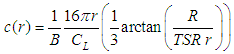
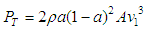
When aircraft wings are designed, the wing is considered to have a uniform velocity distribution along its length and the wing performance is optimal when the angle of attack is set correctly. To optimize wind turbine performance, the pitch angle β must be determined as a function of the blade radius r, and the velocity component in the direction of the rotation plane increases at the positions away from the rotation axis. The ideal blade geometry can be designed according to Schmitz's theory, which allows the generation of the optimal chord length c and pitch angle β considering parameters such as wind speed, blade quantity B, blade radius R, tip-speed ratio TSR, ideal attack angle α and the lift coefficient CL, corresponding to the chosen aerodynamic profile [7]. Equation (1) is used to calculate the pitch angle β and equation (2) is used to calculate the chord length c, both as a function of the radius r [8].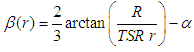 | (1) |
 | (2) |
Characteristics angles, dimensions and the aerodynamic forces produced on the blade with the turbine in operation are indicated in Figure 1. The maximum available power P produced by the wind kinetic energy is given by equation (3), where A is the rotor area and v1 is the wind speed before reaching the turbine. The wind passing through the turbine rotor is decelerated due to the kinetic energy of the wind absorbed by the generator (Figure 2). The turbine mechanical power PT is given by equation (4), where v is the wind speed across through the rotor and v3 is the speed after passing the rotor given by equations (5) and (6). | (3) |
 | (4) |
 | (5) |
 | (6) |
 | Figure 1. Schematic of aerodynamic forces, characteristics angles and rotor dimensions |
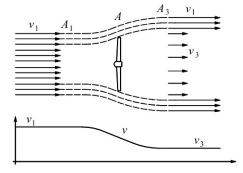 | Figure 2. Wind velocity field around the turbine rotor |
The axial interference factor a, represents the wind speed drop. The wind turbine efficiency can be determined by the dimensionless power coefficient CP, defined by equation (7). The maximum value of the theoretical power coefficient is 0.59, called the Betz limit and reached when a = 1/3. The real power coefficient is always lower than the Betz limit due to system losses such as bearing friction and blade tip vortices. | (7) |
The model was designed to represent a 3 bladed-wind turbine prototype, 100 m tower height and 100 m rotor diameter using a 1: 150 scale. The model specifications are listed in Table 1 and a TSR value of 5 was adopted according to the turbine type and the characteristics of the wind tunnel. Blade machining was done at the CNC Machining Center of the Universidade de Caxias do Sul (UCS).Table 1. Wind turbine specifications
 |
| |
|
Figure 3 shows the main dimensions and characteristics of the model. Figure 4 shows the model mounted on the wind tunnel test section. On the right, it is possible to observe the braking device developed to apply a known torque to the turbine axis. The device has an articulated arm which is driven by a traction spring.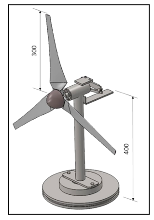 | Figure 3. Dimensions of the wind turbine model |
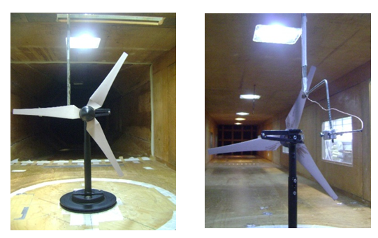 | Figure 4. Turbine model in the wind tunnel |
3. Description of Wind Tunnel Tests
The tests were developed in the “Prof. Joaquim Blessmann” wind tunnel of the UFRGS (Figure 5). The tunnel is of the closed return and boundary layer type. It was designed specifically for static and dynamic testing of structure models, allowing the physical simulation of uniform winds and boundary layer winds. The main test section has a cross-section of 1.2 m × 0.8 m. The maximum velocity of the air flow in this section is 42 m/s [9].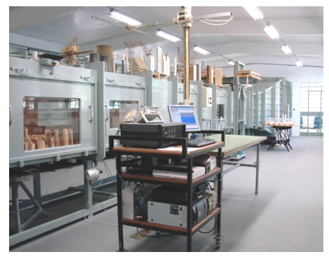 | Figure 5. Prof. Joaquim Blessmann Wind Tunnel – UFRGS |
Measurements of fluctuating velocity were performed with a hot-wire anemometer at different positions leeward to the rotor. Measurements positions are indicated by the x-coordinate. Two types of uniform incident flow were used, one called turbulent wind characterized by a turbulence intensity of 5%, and another called smooth wind characterized by a turbulence intensity minor than 1%. Profiles of mean velocity and RMS values of velocity fluctuations were obtained from these measurements. The model's leeward measurement points ranged from x = 160 mm to 5160 mm. Numerical series of fluctuating velocity were obtained at a sampling frequency of 2048 Hz over a period of 60 seconds. The Reynolds number defined by the test mean velocity and the rotor diameter is 2.25 × 10⁵. The rotor angular velocity was measured at the beginning of the measurements and the mechanical braking system was conveniently fixed to obtain suitable values of the dimensionless parameter TSR. The approximate value of TSR during the tests was 5.
4. Results
In this section, the different results obtained in the described tests are presented. First, mean velocity profiles are indicated at the different measurement points at the leeward of the rotor and, then, the velocity fluctuation profiles are analysed. Vertical and horizontal profiles defined in correspondence to the rotor axis are presented in different positions x.
4.1. Mean Velocity
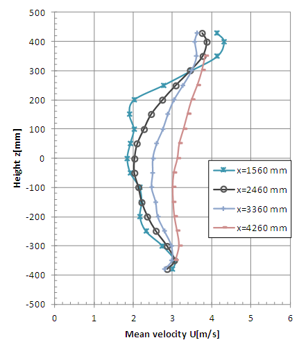
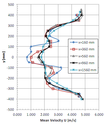
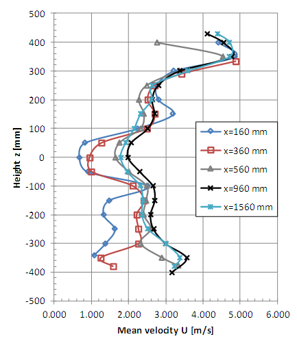
Vertical profiles of mean velocity obtained with turbulent incident flow are presented in Figures 6 and 7. The vertical coordinate z = 0 corresponds to the rotor axis position. Horizontal profiles of mean velocity obtained with turbulent incident flow are presented in Figures 8 and 9, where the horizontal coordinate y = 0 also corresponds to the rotor axis position. Vertical and horizontal profiles of mean velocity obtained with smooth flow are shown in Figures 10, 11, 12 and 13.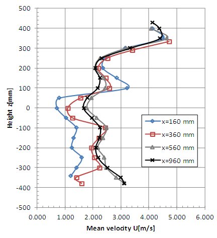 | Figure 6. Vertical profiles of mean velocity with turbulent flow (x = 160, 360, 560 and 960 mm) |
 | Figure 7. Vertical profiles of mean velocity with turbulent flow (x = 1560, 2460, 3360 and 4260 mm) |
 | Figure 8. Horizontal profiles of mean velocity with turbulent flow (x = 160, 360, 560, 960 and 1560 mm) |
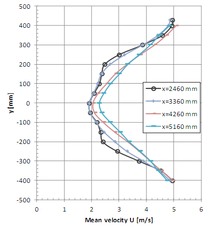
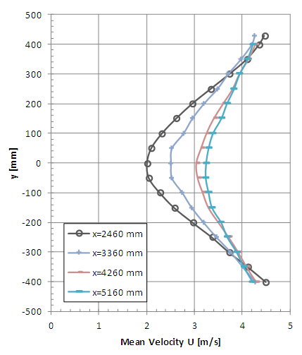 | Figure 9. Horizontal profiles of mean velocity with turbulent flow (x = 2460, 3360, 4260 and 5160 mm) |
 | Figure 10. Vertical profiles of mean velocity with smooth flow (x = 160, 360, 560, 960 and 1560 mm) |
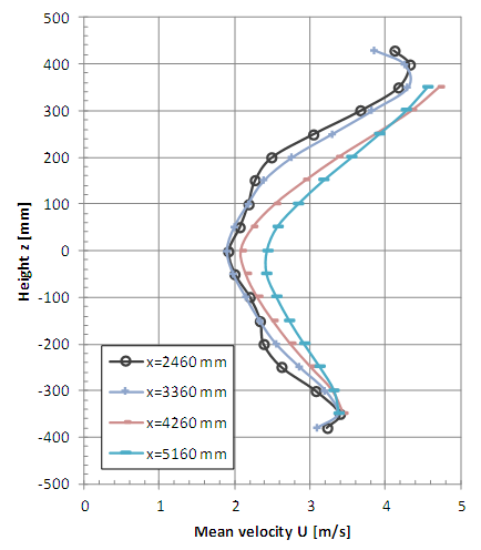 | Figure 11. Vertical profiles of mean velocity with smooth flow (x = 2460, 3360, 4260 and 5160 mm) |
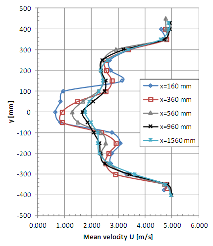 | Figure 12. Horizontal profiles of mean velocity with smooth flow (x = 160, 360, 560, 960 and 1560 mm) |
 | Figure 13. Horizontal profiles of mean velocity with smooth flow (x = 2460, 3360, 4260 and 5160 mm) |
It is possible to observe the complexity of the flow at the measurement positions x = 160, 360, 560 and 960 near the rotor (Figures 6, 8, 10 and 12), even considering that one-channel hot-wire anemometer can only detect the longitudinal component of velocity. The influence of the generator model tower is clearly shown for the non-symmetrical vertical profiles where greater falls of speed are observed in the lower measurement points. The horizontal profiles (Figures 8, 9, 12 and 13) indicate a good symmetry excepting the points close to the braking system (x = 160 mm, z = ±100 mm).
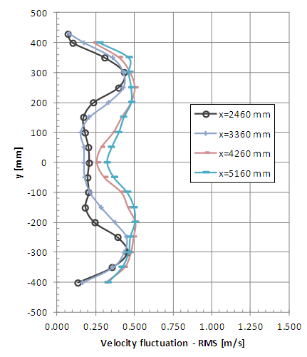
4.2. Fluctuating Velocity
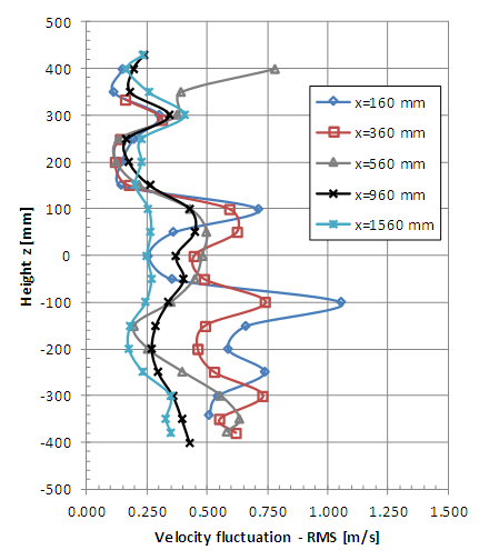
The vertical profiles of the velocity fluctuations indicated in figures 14 and 15 were obtained with uniform turbulent incident flow while the horizontal profiles of figures 16 and 17 also were obtained with turbulent flow. The coordinates y = 0 and z = 0 correspond to the rotor axis. Vertical and horizontal profiles of velocity fluctuations obtained with smooth flow are presented in Figures 18, 19, 20 and 21.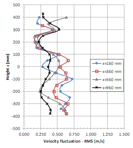 | Figure 14. Vertical profiles of velocity fluctuation (RMS value) with turbulent flow (x = 160, 360, 560 and 960 mm) |
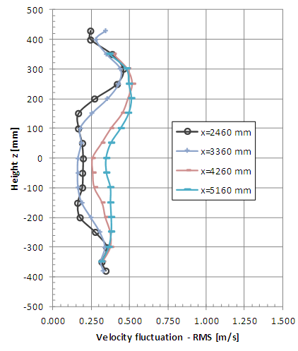
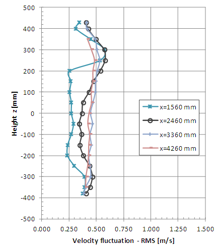 | Figure 15. Vertical profiles of velocity fluctuation (RMS value) with turbulent flow (x = 1560, 2460, 3360 and 4260 mm) |
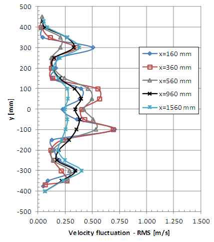
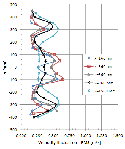 | Figure 16. Horizontal profiles of velocity fluctuation (RMS value) with turbulent flow (x = 160, 360, 560, 960 and 1560 mm) |
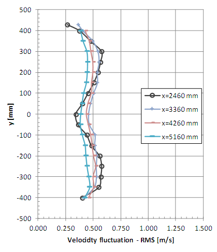 | Figure 17. Horizontal profiles of velocity fluctuation (RMS value) with turbulent flow (x = 2460, 3360, 4260 and 5160 mm) |
 | Figure 18. Vertical profiles of velocity fluctuation (RMS value) with smooth flow (x = 160, 360, 560, 960 and 1560 mm) |
 | Figure 19. Vertical profiles of velocity fluctuation (RMS value) with smooth flow (x = 2460, 3360, 4260 and 5160 mm) |
 | Figure 20. Horizontal profiles of velocity fluctuation (RMS value) with smooth flow (x = 160, 360, 560, 960 and 1560 mm) |
 | Figure 21. Horizontal profiles of velocity fluctuation (RMS value) with smooth flow (x = 2460, 3360, 4260 and 5160 mm) |
The non-symmetrical vertical profiles of velocity fluctuations are also verified indicating the presence of the model column which causes peaks due to the vortex shedding. Therefore, the peaks of fluctuations are greater at the lower points for the measurement positions x = 160 and 360 mm. The horizontal profiles of the fluctuations also show good symmetry but local vortex shedding is observed in the vicinity of the braking device. It is possible to observe greater uniformity of the profiles of RMS values of the velocity fluctuations in the positions farthest from the model when the incident wind is turbulent.
4.3. Discussion of Results
The results indicate more uniform velocity profiles in the case of turbulent incident wind at the farthest positions of the turbine. This behaviour is also verified for fluctuating velocity profiles and would indicate that the re-composition of the flow is faster when the incident wind is turbulent.The complexity of the flow at the measurement points close to the rotor that was observed in the mean velocity analysis also manifests itself in the vortex shedding that indicate the velocity fluctuation profiles.The re-composition of the turbulence levels of the incident flow is not evidenced in these results. Greater turbulence intensity values than the initial ones were obtained in the measurement positions farthest from the turbine. This behavior is the most interesting observation in the analysis of results.
5. Conclusions
The turbine design is carried out based on aerodynamic considerations that simplify the flow configuration passing the rotor. Experimental studies allow to observe the complexity of turbulent wakes generated at the rotor leeward. In particular, this study allows to identify zones of greater complexity from the evaluation of the mean flow and the turbulence levels in the wake of a wind turbine model. The influence of the turbulence of the incident flow is also analyzed from the experimental results. Finally, it can be verified that the re-composition of the average flow does not necessarily imply that the levels of turbulence reached the initial values. In a forthcoming work, the evolution of the turbulence spectra in the wake as a function of the position and leeward distance of the rotor will be analyzed.
ACKNOWLEDGEMENTS
The authors wish to acknowledge the financial support of the Conselho Nacional de Desenvolvimento Científico e Tecnológico – CNPq, Brazil to develop this work.
References
| [1] | Crespo, A., Hernandez, J., Frandsen, S., “Survey of Modelling Methods for Wind Turbine Wakes and Wind Farms”, Wind Energy, 2, 1-24, 1999. |
| [2] | Frandsen, S., Barthelmie, R., Pryor, S., Rathmann, O., Larsen, S., Højstrup, J., Nielsen, P., Thøgersen, M., “Analytical modeling of wind speed deficit in large offshore wind farms”, EWEC 2004, November 22-25, London, UK, 2004. |
| [3] | Bartl, J. “Wake measurements behind an array of two model wind turbines”, Master of Science Thesis, KTH School of Industrial Engineering and Management Energy Technology, EGI-2011-127 MSC EKV 866, Division of Heat and Power Technology, SE-100 44 Stockholm, 2011. |
| [4] | Chamorro, L., Porté-Agel, F. “Turbulent Flow Inside and Above a Wind Farm: A Wind-Tunnel Study”, Energies 2011, 4, 1916-1936, 2011. |
| [5] | Bayatti I., Belloli M., Bernini L., Zasso A. “Aerodynamic design methodology for wind tunnel tests of wind turbine rotors”. J. Wind Eng. Ind. Aerodyn. 167: 217-227, 2017. |
| [6] | Wittwer A., Dorado R., Alvarez y Alvarez G., Degrazia G., Loredo-Souza A., Bodmann B. “Flow in the Wake of Wind Turbines: Turbulence Spectral Analysis by Wind Tunnel Tests”. American Journal of Environmental Engineering. 6: 109-115, 2016. |
| [7] | Thumthae C., Chitsomboon T. “Optimal angle of attack for untwisted blade Wind turbine”. Renewable Energy 34: 1279-1284, 2009. |
| [8] | Gundtoft, S. “Wind Turbines”. University College of Aarhus, - 2° ed. - Dinamarca, 2009. |
| [9] | Blessmann, J. “The Boundary Layer Wind Tunnel of UFRGS”. J. Wind Eng. Ind. Aerodyn. 10: 231-248, 1982. |

 Abstract
 Reference
 Full-Text PDF
 Full-text HTML