Guilherme Luís Mello Ribeiro1, Fabricio Pereira Härter1, Régis Sperotto de Quadros1, Daniela Buske1, Otávio Medeiros2
1Programa de Pós-Graduação em Modelagem Matemática, Universidade Federal de Pelotas, Pelotas, Brasil
2Faculdade de Meteorologia, Universidade Federal de Pelotas, Pelotas, Brasil
Correspondence to: Daniela Buske, Programa de Pós-Graduação em Modelagem Matemática, Universidade Federal de Pelotas, Pelotas, Brasil.
| Email: |  |
Copyright © 2018 The Author(s). Published by Scientific & Academic Publishing.
This work is licensed under the Creative Commons Attribution International License (CC BY).
http://creativecommons.org/licenses/by/4.0/

Abstract
The present work deals with the initialization of the WRF model by the digital filter. That technique is used to filter high-frequency gravity waves. High-frequency gravity waves arise due to the imbalance between the pressure and wind fields in the model initial condition and tend to spread through the domain. The imbalance causes between the pressure and wind fields are varied, such as: error in the observed data, imperfection of the numerical method that discretizes the differential equations by finite differences, grid resolution, difficulty to represent the nonlinear terms of the equations of the model and the truncation error in spectral models. In the generation of the filtered time series, oscillations occur close to the cut-off frequency (Gibbs oscillations), which are smoothed with the use of so-called window functions. In the proposed methodology, it is described the operation of the digital filter and the most efficient window function, according to a literature (Dolph-Chebyshev). Different cut-off frequencies, serial sizes, window functions and initialization shapes are also investigated to generate the filtered series. In addition, the results are explored through the simulation of a explosive cyclogenesis case that occurred on 03/01/2014. The results demonstrate that the model simulated the cyclogenesis, when compared to CPTEC analyzes (used as reference). The digital filter showed an efficient methodology for the WRF initialization, with nested grids. The best results were obtained with 1-hour cut-off frequency, 1-hour series, Dolph-Chebyshev window function and TDFI integration estrategy.
Keywords:
Low-pass filter, Numeric model, Gravity waves
Cite this paper: Guilherme Luís Mello Ribeiro, Fabricio Pereira Härter, Régis Sperotto de Quadros, Daniela Buske, Otávio Medeiros, WRF Model Initialization Applied to a Case of Explosive Cyclogenesis Case in the Southern Region of Brazil, American Journal of Environmental Engineering, Vol. 8 No. 4, 2018, pp. 88-98. doi: 10.5923/j.ajee.20180804.02.
1. Introduction
Numerical time prediction models, such as the WRF, show spurious oscillations (noise) generated by high frequency gravity waves in the first hours of integration. These oscillations, which arise due to the imbalance between the pressure and wind fields in the model initial condition, and tend to spread through the domain, degrading the forecast.The imbalance that arises between the pressure and wind fields has several causes, such as: error in the observed data, imperfection of the numerical method that discretizes the differential equations by finite differences, grid resolution, difficulty in representing the equations nonlinear weights and truncation error.In order to reduce this imbalance between the pressure and wind fields in the model initial condition, initialization techniques emerge, such as digital filtering.These techniques eliminate or attenuate waves that are not physical solutions of the model equations. Thus, the digital filter in WRF is a low pass filter applied to the model fields time series. The time series are generated through three possible forms of integration: adiabatic (backward integration), diabatic (forward integration) and the combination of the two integration techniques.More recently, with the emergence of data assimilation systems, the digital filtering technique has been cited as an integral and indispensable part of the use of these systems.The main objective of this work is to accelerate the balance between the pressure and wind fields in the WRF initial condition. In addition and more specifically, we intend to: evaluate the performance of digital filtering initiation (DFI) applied to the model with nested grids, investigate the methodology with respect to different cut-off frequencies, series size, window functions and integration strategies and to explore the results through a explosive cyclogenesis case that occurred in the South Atlantic on 03/01/2014, as a form of validation of the technique.This paper is divided into five sections. The first section, as seen, is show the introduction. In the second section, there is a brief literature review, followed by the third section, where the methodology is highlighted and the fourth and fifth sections are reserved for results and conclusions, respectively.
2. Literature Review
The first techniques of initialization of numerical models of time arose in 1960 with [1], who concluded that the work with models of simplified equations would be the best form of reduction of noise in the meteorological modes, due to the computational limitations characteristic of the time. Since then, the initialization strategies have been evolving, and the main references should be mentioned.[2] used the Laplace transform initialization technique to initialize the data of a barotropic prediction model over a limited area. This methodology was successful in suppressing high frequency oscillations in the first few hours of forecasting, during which time the greatest impacts of this technique were verified.[3] applied the digital filtering technique to initialize data from the High Resolution Limited Area Model (HIRLAM). The method uses the digital filter applied to the time series of model variables, generated by backward and forward integrations, from the initial time, and a satisfactory initialization scheme was shown, when compared to the Initialization pattern by Normal Non-linear Modes (INNM), used in the HIRLAN model. The main appeal of the technique is the ease of implementation.[4] implemented the digital filter in the spectral model of primitive equations, used operationally at the Canadian Meteorological Center (CMC). In this work, digital filtering initialization was compared to an experiment in which the pressure and wind fields were in balance and initialization by normal non-linear modes in a cycle of assimilation of radiosonde data. The authors verified the superiority of DFI in relation to INNM and its similarity with respect to the experiment in which the fields of pressure and wind were in balance.[5] combined the assimilation technique known as Newtonian relaxation with DFI, in order to obtain initial conditions for the Japanese Limited Area Model (LAM). The authors corrected the LAM forecast by assimilating the analyzes generated by the global model of the NCEP. In addition, the application to LAM shows that the scheme is efficient, low computational cost and control of Gibbs oscillations.[6] developed a WRF initialization study by digital filter at the Chinese Institute of Urban Meteorology (IUM). Tests without the use of the digital filters showed high levels of noise, but when the model was initialized with the filter, with a resolution of 9 km and an integration cycle of three hours, we observed the damping of fast waves.[7] performed some tests in version 3.0 of the WRF. Basically, real-time predictions were performed with and without the use of the technique digital filtering, with the difference that the filtering cycle is used twice (integration forwards and backwards) [8] and [9]. As the authors report, this experiment presented quite satisfactory results, as the gain trend in precision of the variable surface pressure, which presented small oscillations during the first two hours of digital filtering.[10] evaluated the performance of DFI with different window functions, applied to remove the Gibbs oscillations: (i) Blackman; (ii) Dolph; (iii) Dolph-Chebyshev; (iv) Hamming; (v) Kaiser; (vi) Lanczos; (vii) Potter; (viii) recursive and (ix) uniform. The technical analysis of these functions suggest the superiority of the Dolph-Chebyshev (DC) window in relation to the others. The authors also describe that digital filtering initialization techniques are implemented in WRF: (i) Diabatic digital filtering; (ii) Adiabtic digital filtering and (iii) Combined digital filtering (forward and backward integration). In this sense, the tests carried out in the Tehran region of Iran, with a grid of 45 x 45 km, demonstrated the superiority of the combined digital filtering technique associated the Dolph-Chebyshev window. This approach presented it is efficiency in the first three hours of integration, which meets the needs of the forecast model, which presents the highest noise in this period.[11] evaluated the DFI associated with the data assimilation system of the WRF version 3.0.1.1. The DFI was used with a Dolph-Chebyshev window function and combined integration (TDFI) (1 h forwards and backwards). The assessment of this study, in the northern region of the United States, concluded that there were no significant improvements in the forecast, especially with regard to temperature, but there were improvement in wind fields.[12] studied the DFI coupled to the WRF through the Rapid System Refresh (RAP), which replaced the Rapid Update Cycle (RUC), associated with the ARW of WRF since 2012 at National Oceanic and Atmospheric Administration (NOAA)/National Center for Environmental Prediction (NCEP). In this study, the authors report the use of DFI with forward integration, highlighting the essentiality of its utilization data assimilation due to the simplicity and effectiveness of attenuating high frequency waves (noise) during the initial integration period of the model.[13] also evaluated the DFI associated with RAP, concluding of the need to use the DFI in the NOAA/NCEP data assimilation system. The results of the evaluation carried out, including evaluating the weights of the coefficients of with the Dolph-Chebyshev window, demonstrated the effectiveness of the DFI in attenuate the high frequency waves, evidencing the reduction of errors in the mass and momentum fields in the initial period of integration of the model. However, the authors observed a decrease in convection generated, inconsistent with reality.Based on the studies of [14], [10] and [13], it is assumed that the approach of the function Dolph-Chebyshev window would present the best results. According to first author, this window function presents all the characteristics verified in an optimal filter because it minimizes the differences between the filter transfer function and the transfer band stop function. The second author reiterates this superiority of said window function, since unwanted fluctuations, in the tests performed, were eliminated in the first three hours. Moreover, comparing the precipitation data observed per station with the forecast results carried out with initialization using the Dolph-Chebyshev window and diabatic integration strategy, it was verified that the filter prediction has a reduction of the mean square error in relation to prediction without filter. The third author highlights that, in spite of the problem of attenuation of the convection parameters in the utilization combined integration (TDFI) and Dolph-Chebyshev window function reduction of high frequency waves and errors.
3. Methodology
In this chapter, is presented the digital filter, the Dolph-Chebyshev window function and others window functions (use to reassemble Gibbs oscillations) implemented in WRF. In addition, we investigate the best parameters for the use of the DFI in WRF 3.8 version and describes the case of explored in this work.
3.1. The Digital Filter
The digital filter employed in the WRF consists of a low-pass filter, where frequencies above of the cut-off frequency (CF) are eliminated. These frequencies that are positioned in a range above of the cut tend to spread through the model domain and degrade the forecast. In this sense, the digital filter is a convolution between two functions, as seen in 1.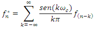 | (1) |
Where  are the input data;
  are the output data and
  is the cut-off frequency.But in pratical problems, the digital filter is applied to a finite sequence, which introduce the Gibbs oscillations close to the cut-off frequence. Some window functions have been proposed to resolve this problem. Thus, the new sequence filtered with 2N+1 elements is given by 2.
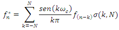 | (2) |
Where the parameter  is the control factor of the Gibbs oscillations, also called window function.
3.2. The Dolph-Chebyshev Window Function
The Dolph-Chebyshev window function was constructed based on the Chebyshev polynomials, and the first time used by Dolph in the 1946 in development of a radio antenna with optimal directional characteristics [8]. In this sense, the Dolph-Chebyshev window function with size 2M+1 is 3. | (3) |
Where  is the reason between of the lateral wall amplitude and the main wall amplitude.
  is described by 4 and
  is the Chebyshev polynomial of order
  defined in 5.
 | (4) |
 | (5) |
3.3. Other Window Functions Implemented in WRF
In addition to the Dolph-Chebyshev window function, eight other window functions were implemented in the WRF: Blackman, Dolph, Hamming, Kaiser, Lanczos, Potter, Recursive and Uniform.
3.4. Integration Strategies Implemented in WRF
The WRF dynamic ARW solver supports three different integration strategies, to generate the filtered temporal series: Digital Filter Launch (DFL), Diabatic Digital Filter Initialization (DDFI) and Twice Digital Filter Initialization (TDFI).The DFL strategy [15] generates the time series by forward integration, with all physical and diffusive parameters enabled (diabatic integration), from the initial point (t = 0) for 2N time steps. Filtering starts at the starting point (t = 0) and the forecast starting point is in N time steps. To generate the time series, the DDFL strategy [17] starts with an adiabatic integration, starting from the initial point (t = 0) to -N time steps (backward integration). After, the scheme performs diabatic integration (with all physical and diffusive parameters enabled) from -N to N time steps during the filtering occurs. The forecast start is at the same starting point (t = 0). In adiabatic integration, the physical and diffusive parameters are disabled.Finally, the TDFI strategy [15] involves two applications the digital filter. It begins with an adiabatic integration, from the initial point (t = 0) to -2N time steps, during which the first filtering is applied. After, starts in -N a diabatic integration (with all the physical and diffusive parameters enabled) to N time steps, during which the second filtering is applied. Gives same way as in the DDFI scheme, the forecast starts at (t = 0) and integration adiabatic the physical and diffusive parameters are disabled.The Figure 1 demonstrates the three integration strategies.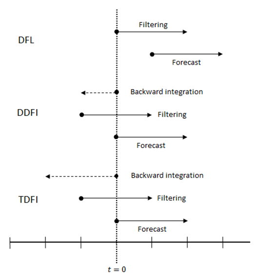 | Figure 1. Integration strategies implemented in WRF. (Source: Adapted from [14]) |
3.5. The Case Study
The synotic analysis is based on CPTEC-GPT (www.cptec.inpe.br) and GOES-13 satellite images on the thermal infrared channel. Subsequently, in section 4, the WRF model ability reproduce the CPTEC-GPT is evaluated.In the highlighted image of GOES-13 at 06 and 12 UTC on 03/01/2014 (Figure 2 (a-b)) the formation of cold clouds and with high top extending from Rio Grande do Sul (RS) state to the South Atlantic Ocean, where they present cyclonic curvature. These clouds with precipitation potential travel from southwest to northeast, and at 18 UTC on 03/01/2014 and 00 UTC on 04/01/2014 they are on Santa Catarina (SC) and southern Paraná (PR) (Figure 2 (c-d)), suggesting possibility of precipitation in these states.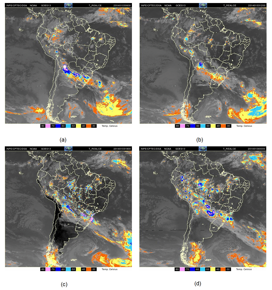 | Figure 2. Highlighted image of the Goes-13 satellite, in the thermal infrared channel at: (a) 06 UTC (03/01/2014); (b) 12 UTC (03/01/2014); (c) 18 UTC (03/01/2014); (d) 00 UTC (04/01/2014). (Source: CPTEC) |
Figure 2 shows the atmospheric configuration at 06, 12 and 18 UTC on 03/01/2014 and 00 UTC on 04/01/2014. The fields in figure 3 refer to surface (a), at 850 hPa (b) at 500 hPa (c) and 250 hPa.Although the area of interest in this work is the South Atlantic and Brazil South Region (BSR), is showing the large-scale panorama on Brazil, to situate the reader on the systems synoptic that cause weather changes during the study period.Figure 3 (a) shows an important intertropical convergence zone recognition mechanism in the northern and northeastern regions of Brazil, a northern region of the country. It is also observed a subtropical high in the South Pacific and a low pressure system in 53° S/58° W. Particularly important for this study, is a presence of the extratropical cyclone with a center of 996 hPa, in the South Atlantic, one southeast of RS, specifically in 40° S/47° W, associated with a cold front with the cold arm entering the RS and a baroclinic trough at 250 hPa.At 850 hPa, Figure 3 (b) stands out the low-level jet, which carries heat and humidity of the Amazon to the south of the country and feeds the instability in the south of RS.At the mean levels, 500 hPa, Figure 3 (c), the zonal flow is observed with a trough prominent, according to the geopotential lines (white on the map). This one is associated with the advection of cyclonic relative vorticity, convection and precipitation on its east side. The inclination of the trough axis relative to the surface shows that the system is baroclinic, similar those identified by [17].Fields at high levels (250 hPa - Figure 3 (d)) show the subtropical jet (SJ) (dashed thick red line) and the polar jet (PJ) (dashed thick orange line). This region of strong winds migrates towards lower latitudes as the cold enters the continent and, for this reason, helps to predict the spread of fronts. When positioned at latitudes lower than 30° S, it prevents the flow from the north deviated by the Andes transporting warm and moisture Amazon rainforest at BSR. In this case, the jet should not be sufficient for the north to prevent that the northern outflow reaches at BSR. This observation is confirmed by the current line field (solid blue line), which shows the low-level jet carrying heat and moisture from north to south of the country.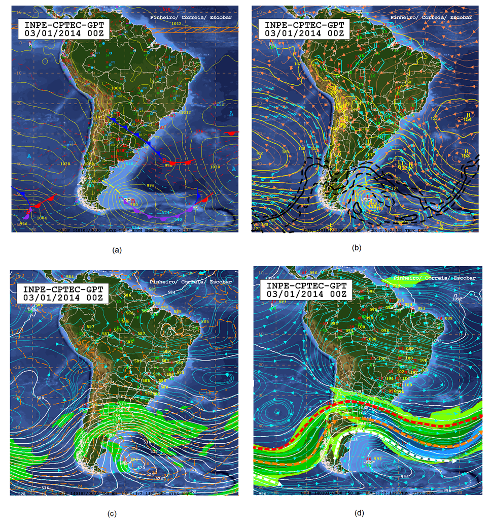 | Figure 3. Product CPTEC-GPT at 00 UTC (03/01/2014): (a) Surface Chart; (b) Height Chart – 850 hPa; (c) Height Chart – 500 hPa; (d) Height Chart – 250 hPa. (Source: CPTEC) |
In summary, an analysis shows a classic case of explosive cyclogenesis (EC) studied by [18], formed in the region under analysis. The cyclone is associated with the formation of the cold front that spreads from west to east through a Rossby wave, in a baroclinically unstable atmosphere.The consequences of this cyclogenesis were strong winds and high precipitation as reported in the newspapers (www.dc.clicrbs.com.br).
3.6. Domain Study
For the elaboration of the simulations, it was necessary to establish the area of study and the time interval in which the model performs the integrations. Therefore, two domains were defined, predicting the tests with nested grids. In that this sense, a larger domain was delineated, with a grid of 27 km and a nested one, with a grid of 9 km. Regarding the time step, 180 s were delimited for the larger grid and 60 s for the smaller grid. It should be noted here, that the model is rotated in the hydrostatic mode on the larger grid and non-hydrostatic on the smaller grid. Said domains were characterized as domain 1 and domain 2 and their ranges are exemplified in Figure 4.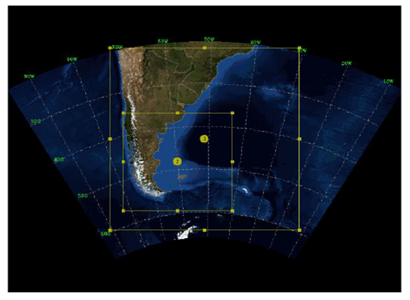 | Figure 4. Domain study: domain 1 – external grid and domain 2 – internal grid |
4. Results and Discussions
In this chapter, the performance of the proposed both method is evaluated. At section 4.1, it is checked whether the simulation reproduces the synoptic scene described in the product CPTEC-GPT. At section 4.2 is defined the variable that the filtering efficiency in eliminating spurious oscillations. Section 4.3 investigates which cut-off frequency (CF) will be applied to the filter. Once this important parameter is defined, in the section 4.4, where evaluated the size of the series applied in the filtering process. Defined CF and size of the series, we investigate in section 4.5 the window function that best attenuates the Gibbs oscillations. In Section 4.6, we investigate different model integration strategies in the filtering process. At the end of the chapter, in section 4.7, it is evaluated whether initialization applies the conditions of an efficient initialization scheme, according to [3].
4.1. Simulation without Digital Filtering
In this section, we present the case simulation without the digital filter, so that check if the WRF model can reproduce the synoptic systems presented by the CPTEC-GPT product on 01/03/2014. It can be seen that in the field at the Mean Sea Level Pressure (MSLP) (00 UTC of 03/01/2014), Figure 5 (a-b), the WRF reproduces the low pressure system in 53° S/58° W with nucleus at 975 hPa in domain 1 and 976 hPa in domain 2 and a extratropical cyclone in formation at 40° S/47° W with nucleus at 995 hPa in the domain 1. That is, the low-pressure system predicted by the WRF is more intense and delayed (more to the south) in relation to product CPTEC-GPT, assuming greater advection of thickness and less advection of vorticity. With respect to the extratropical cyclone almost exact reproduction of the WRF compared with the product concerned. It is necessary to inform that the advection of vorticity is responsible for the propagation of the system and the advection of thickness is responsible for the amplification and decay of the system.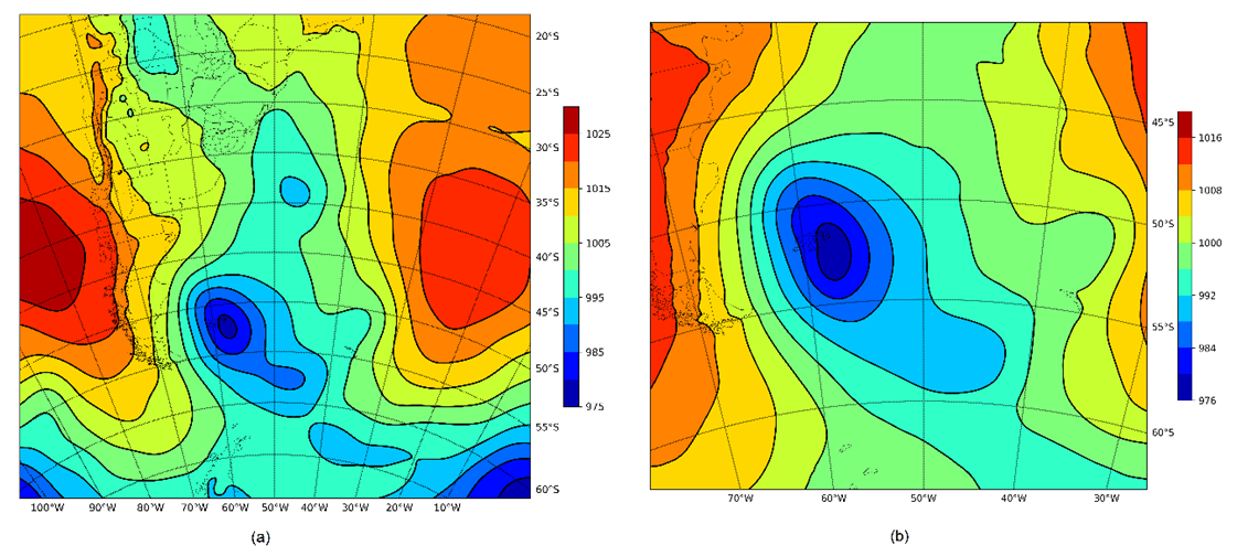 | Figure 5. MSLP (hPa) 00 UTC (03/01/2014) – Analysis without DFI for domain 1 (a) and for domain 2 (b) |
In Figure 6 (a-b), the 12-hour MSLP prediction field confirms decay of the extratropical cyclone low center at 46° S/ 38° W with nucleus at 972 hPa in domain 1 and 970 hPa in domain 2, and weakening of the low pressure system at 50° S/ 55° W with nucleus at 978 hPa at domain 1 and 975 hPa at domain 2. In this sense, the explosive characteristic of the extratropical cyclone is clear, since the MSLP decreased by 23 hPa in a period of 12 hours, which corresponds to 1, 15 Bergeron for the mean latitude of the displacement (46°). Therefore, we conclude the same as in [19], that is, the extratropical cyclone in formation is actually the one that has the explosive characteristic and that actually reached the region of interest and not the low-pressure system, which is in the phase of weakening.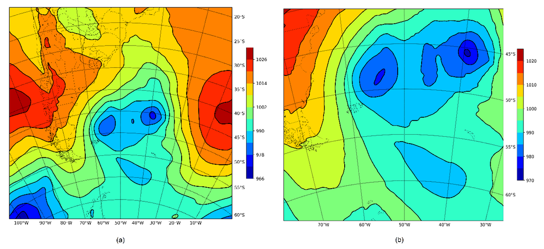 | Figure 6. MSLP (hPa) at 12 UTC (03/01/2014) – Forecast without DFI for domain 1 (a) and for domain 2 (b) |
4.2. Mean Absolute Surface Pressure Tendency (SPT)
In order to evaluate the application of DFI and its ability to remove spurious oscillations, it was verified that the model reproduced the active systems in the simulated period, evidencing the cyclogenesis in the South Atlantic, according to [19]. However, before applying the DFI, it is necessary to define the following filter parameters: cut-off frequency (CF), serial size to be filtered, window function and integration strategy. In this sense, were plotted the time evolution of the Mean Absolute Pressure Surface Tendency (SPT), variable that provides the total integrated noise in the layer over the domain, according to 6.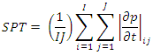 | (6) |
Where  is pressure
  and
and  is time
4.3. Cut-off Frequency Investigation
Once the SPT variable was defined, the DFI was evaluated with a 1-hour series for cut-off frequency (CF) of 7,5 minutes, 15 minutes, 30 minutes and 1 hour, Dolph- Chebyshev window function (DC) and TDFI integration. The attenuation in SPT is observed with all CF, compared to the uninitialized scheme, and the CF of 1 hour presents best result. This effect is reproduced in both domain 1 and domain 2, although in domain 1 the attenuation was higher. The result of this experiment is shown in Figure 7 (a-b). It should be noted that, in the following graphs, the time (in hours h) is plotted on the abscissa axis and on the ordinates axis is plotted the SPT (in hectopascal hPa).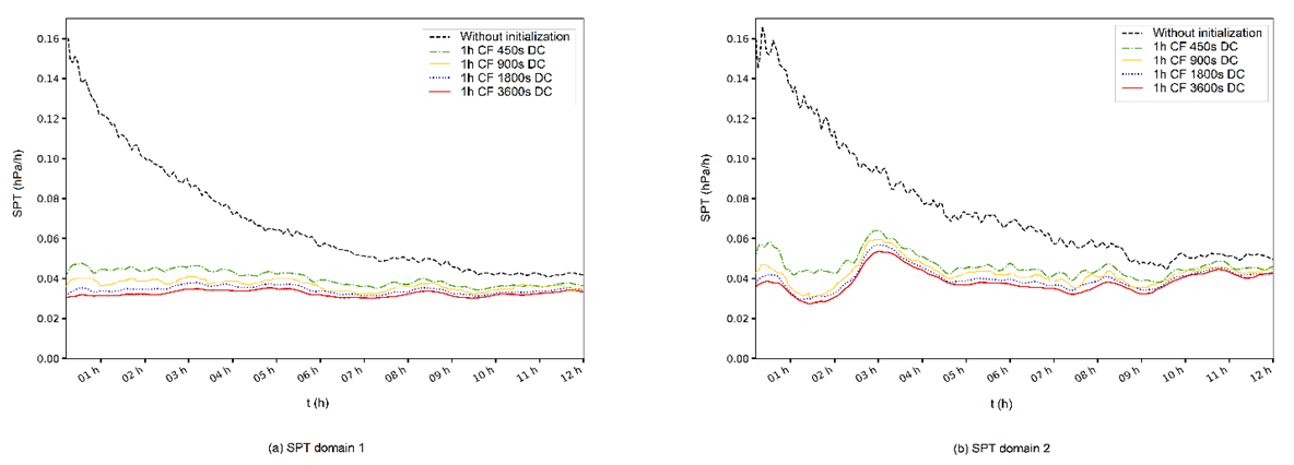 | Figure 7. SPT (hPa/h) – (a-b) domain 1 and 2 – black dashed line (without initialization), green dashed line (CF 7,5 min, 1h series, DC window and TDFI integration), solid orange line (CF 15 min, 1h series, DC window and TDFI integration), dotted blue line (CF 30 min, 1h series, DC window and TDFI integration) and solid red line (CF 60 min, 1h series, DC window and TDFI integration) |
4.4. Size of the Series to be Filtered Investigation
Once the CF to be used is defined, the size of the variable series applied in the filtering, since there is a direct implication between the size of the series and the computational cost of the DFI. For that, simulation with CF of 1 h and series generated by 1, 2, 3 and 4 hours of integration, Dolph-Chebyshev window function (DC) and TDFI integration were performed. This is shown in Figure 8 (a-b). For both domain 1 and domain 2, the attenuation of the SPT in all series, compared to the uninitialized scheme. The efficiency similarity of all series sizes is still visualized. However, the superiority of the 1-hour series is demonstrated, since it presents lower oscillations in the SPT and because it requires a lower computational cost to be generated.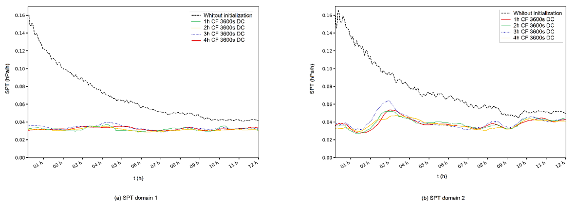 | Figure 8. SPT (hPa/h) – (a-b) domain 1 and 2 – black dashed line (without initialization), solid red line (CF 1h, 1h series, DC window and TDFI integration), solid green line (CF 1h, 2h series, DC window and TDFI integration), dotted blue line (CF 1h, 3h series, DC window and TDFI integration) and solid red line (CF 1h, 4h series, DC window and TDFI integration) |
4.5. Window Function Investigation
Defined CF and series size, one investigates among the window functions implemented in the WRF, which better reduces Gibbs oscillations. In Figure 9 (a-b), the integrations with the windows functions implemented in WRF: Blackman; Dolph; Dolph-Chebyshev; Hamming; Kaiser; Lanczos; Potter; Recursive and Uniform.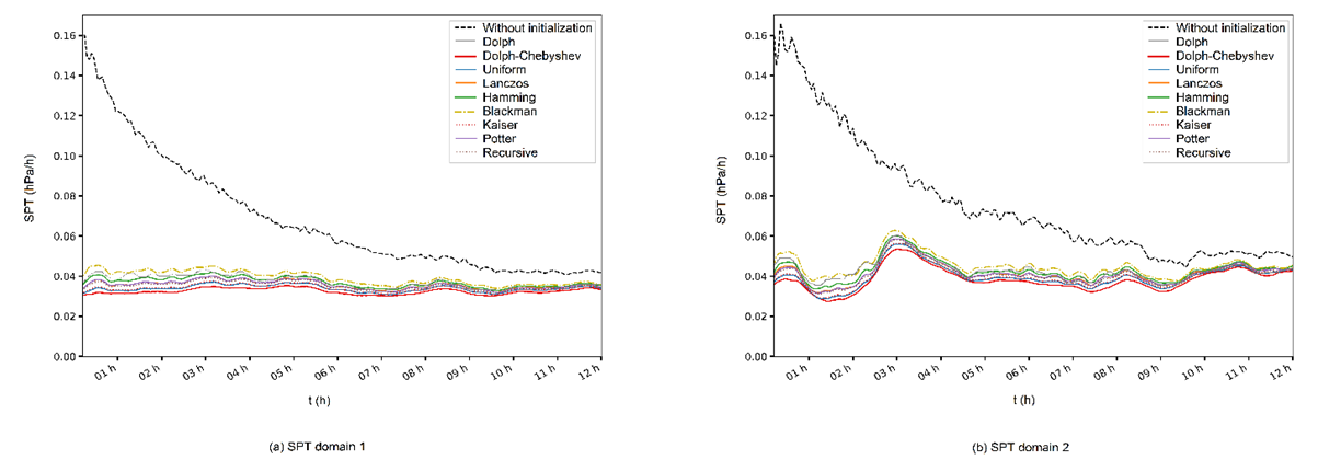 | Figure 9. SPT (hPa/h) – (a-b) domain 1 and 2 – black dashed line (without initialization), solid grey line (Dolph), solid red line (Dolph Chebyshev), solid blue line (Uniform), solid orange line (Lanczos), solid green line (Hamming), dashed yellow line (Blackman), dotted lilac line (Kaiser), solid purple line (Potter), dotted brown line (Recursive) |
The result of the simulation demonstrated the efficiency of the DFI in the entire functions window, when compared to the scheme without initialization. However, is demonstrated the superiority of the Dolph-Chebyshev window function, because it presents less noise during the model integration, in the two domains.
4.6. Integration Strategy Investigation
In this section, we tested the integration strategies DFL, DDFI and TDFI, with the previously made definitions, that is, CF of 1 h, series of 1 h and Dolph-Chebyshev window function. The results of simulation are presented in Figure 10 (a-b).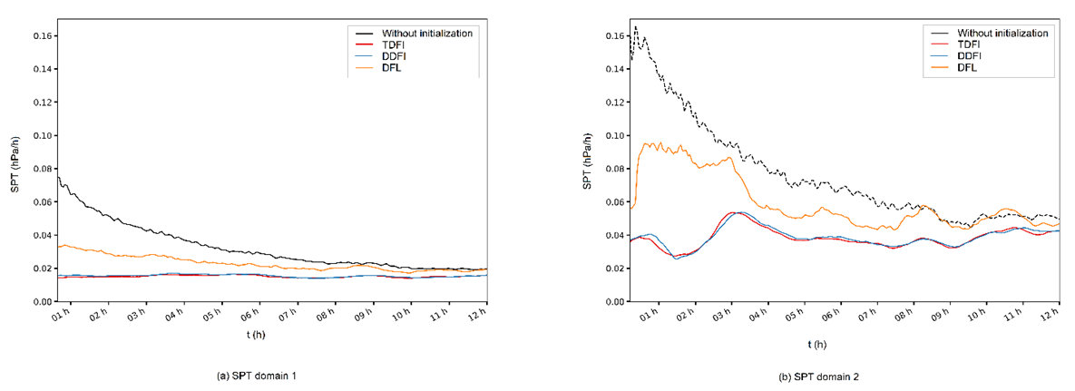 | Figure 10. SPT (hPa/h) – (a-b) domain 1 and 2 – black dashed line (without initialization), solid red line (TDFI), solid blue line (DDFI), solid orange line (DFL) |
Analyzing the results, it is verified the superiority of the strategies of TDFI and DDFI integration, in relation to the uninitialized scheme and the DFL strategy. However, due to the similarity of performance of the TDFI and DDFI strategies in the case study, it was decided to follow the literature [11] and [14], which indicate the superiority of the TDFI strategy. This result is extensive to the two domains studied.The analysis of the results of sections 4.3-4.6, allows to observe which DFI parameters presented the best results in the WRF model, for the case studied, being they: (i) cut-off frequency of 1 h; (ii) series of 1 h; (iii) Dolph-Chebyshev window function and (iv) TDFI integration strategy.
4.7. The Digital Filtering Performance Analysis
The analysis of the previous sections supports the conclusion about the best parameters to initialize the WRF model: (i) cut-off frequency of 1 h; (ii) series of 1h; (iii) Dolph-Chebyshev window function and (iv) TDFI integration strategy.However, according to [3], an efficient initialization system must have three essential characteristics: (i) removes high-frequency oscillations from the forecast; (ii) does not degrade the forecast and (iii) the changes made in the initial fields are acceptably small.In this sense, in order to evaluate the three essential characteristics of an efficient initialization scheme, the subtraction between the fields with and without DFI were generated for the two domains, which is shown in Figure 11 (a-b).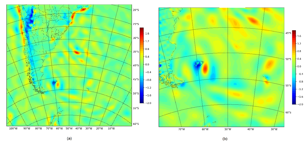 | Figure 11. MSLP (hPa) at 00 UTC (03/01/2014) – Difference of analysis with and without DFI for domain 1 (a) and domain 2 (b) |
First, from the results obtained with the temporal evolution of the variable SPT, it is verified that the DFI satisfies the first essential condition for an efficient system, according to [3], because the noise levels were attenuated in all simulations.Based on results obtained in Figure 11 (a-b), where obtained the MSLP fields of analysis differences, with DFI, in both domains, it is concluded that the use meets the second and the third conditions for an efficient system, according to [3], since the forecast was not degrade and the changes made in the initial fields were really small, allowing to evaluate that the initialization system used in this study is an efficient system, according to the mentioned authors.
5. Conclusions
The DFI, used as the initialization system, must satisfy the conditions of an efficient system: (i) filtering high frequency gravity waves; (ii) not degrade the forecast, and (iii) the changes generated in the initial fields should be small. To evaluate the performance of the DFI in the WRF model, it was proposed to simulate a case of EC occurred on 01/03/2014. This case was characterized by considerable losses materials in Santa Catarina state, caused by strong winds and high levels of precipitation.Therefore, simulations were made to assign the optimal parameters to the DFI application. In the first one, the WRF ability to reproduce the EC on 03/01/2014, where it was concluded that this model reproduced satisfactorily the low pressure system that reached the south of South America and South Atlantic and almost exactly the extratropical explosive cyclone that reached Santa Catarina state, both in comparison to the product CPTEC-GPT. In simulations, the aim was to identify the optimal parameters for the use of the DFI in the WRF. CF was initially investigated, with DFI being evaluated with a 1 h series for cut-off frequencies of 7,5; 15; 30 and 60 min, Dolph-Chebyshev window function and TDFI integration strategy, which allowed us to observe that the cut-off frequency of 1 h presents the best result. Then, once the CF was defined, the size of the time series was analyzed, with CF of 1 h, DC window, TDFI integration strategy and series generated by 1, 2, 3 and 4 h. From this simulation, it was concluded that the series of 1 h presents better performance. After defining the CF and the serial size, we investigated the performance of the nine window functions implemented in the WRF, with TDFI integration strategy. The Dolph-Chebyshev window function proved to be more efficient at removing noise. Finally, defined the CF, the serial size and the window function, the three integration strategies of the filtered time series implemented in the model were analyzed, leading to the conclusion that the TDFI strategy presents the best performance.In conclusion, the WRF model was able to reproduce the EC with nested grids and the DFI technique proved to be efficient in dampening spurious oscillations, as in [7], [10] and [13]. Although the system has the requirements of an efficient starting system, such as high frequency gravity waves, it does not degrade the forecast and as changes generated in the fields are small originators.Finally, we conclude that the main contributions of this work are: (i) to provide, through scientific experimentation, reference parameters for all users of the WRF and (ii) show that initialization, applied to the larger grid, also reduces the noise generated in the smaller grid, but with less intensity, because the smaller grid is generated with greater interpolation, one of the sources of fast gravity waves.
References
| [1] | J. Chaney. The use of the primitive equations of motion in numerical prediction. Tellus, v. 7, n. 1, p. 22-26, 1955. |
| [2] | P. Lynch. Initialization of a barotropic using the Laplace transform technique. Monthly Weather Review. v. 113. n. 8, p. 1338-1344, 1985. |
| [3] | P. Lynch, X. Huang. Initialization of the HIRLAN model using a digital filter. Monthly Weather Review. v. 114. n. 8, p. 1945-1955, 1991. |
| [4] | L. Fillion, H. Mitchell, H. Ritchie, A. Histaniforth. The impact of a digital filter initialization technique in a global data assimilation system. Oceanographic Literature Review. v. 1, n. 43, p. 15, 1996. |
| [5] | V. Innocentini, A. Caetano, F. P. Härter. A first-guess field produced by merging digital filter and nunudging techniques. Revista Brasileira de Meteorologia. v. 17, n. 2, p. 125-140, 1992. |
| [6] | X. Huang, M. Chen, W. Wang, J. Kim, W. Skamarock, T. Henderson. Development of a digital filter initialization for WRF and it is implementation at IUM. 8th Annual WRF user’s workshop, 2007. |
| [7] | T. Smirnova, S. Peckham, S. Benjamin, J. M. Brown. Implementation and testing of WRF digital filter initialization (DFI) at NOAA/Earth System Research Laboratory. Conference of Weather Analisys and Forecasting. v. 23, n. 19, p. 10-21, 2009. |
| [8] | P. Lynch. The Dolph-Chebyshev window: A simple optimal system. Monthly Weather Review. v. 125. n. 4, p. 655-660, 1997. |
| [9] | X. Huang. X. Yang. A new implementation of digital filter inialization schemes for HIRLAM. HIRLAM-5 Project, 2002. |
| [10] | K. Asharafi, M. Azadi, S. Sabetghadam. Effects of various digital filters initialization methods on results of weather research and forecasting (WRF) model. Iranian Journal of Geophysics, v. 5, n. 1, p. 16-33, 2011. |
| [11] | B. C. Ancell. Examination of analysis and forecast errors of right-resolution, bias removal, and digital filter initialization with an ensemble Kalman filter. Monthly Weather Review, v. 140, n. 12, p. 3992-4004, 2012. |
| [12] | K. Zhu, Y. Pan, M. Xue, X. Wang, J. S. Whitaker, S. G. Benjamin, S. S. Weygandt, A. Hu. A regional GSI-based ensemble Kalman filter data assimilation system for the rapid refresh configuration: Testing at reduced resolution. Monthly Weather Review, v. 141, n. 11, p. 4118-4139, 2013. |
| [13] | S. E. Peckham, T. G. Smirnova, S. G. Benjamin, J. M. Brown, J. S. Kenyon. Implementation of a digital filter initialization in the WRF model and its application in the Rapid Refresh. Monthly Weather Review, v. 144, n. 1, p. 99-106, 2016. |
| [14] | W. C. Skamarock, J. B. Clemp, J. Dudhia, D. O. Gill, D. M. Barker, W. Wang, J. G. Powers. A description of the advanced research WRF version 2. DTIC Document, 2005. |
| [15] | P. Lynch, X. Y. Huang. Diabatic initialization using recursive filters. Tellus, v. 46, n. 5, p. 583-597, 1994. |
| [16] | X. Y. Huang, P. Lynch. Diabatic digital filtering initialization: Aplication to the HIRLAM model. Monthly Weather Review, v. 121, n. 2, p. 589-603, 1993. |
| [17] | M. A. Gan, V. B. Rao. Surface cyclogenesis over South America. Monthly Weather Review, v. 119, n. 43, p. 15, 1996. |
| [18] | M. R. Sinclair. A climatology of cyclogenesis for the Southern Hemisphere. Monthly Weather Review, v. 123, n. 6, p. 1601-1619, 1995. |
| [19] | V. D. Avila, A. B. Nunes, R. C. M. Alves. Análise de um caso de ciclogênese explosiva ocorrido em 03/01/2014. Revista Brasileira de Geografia Física, v. 9, n. 4, p. 1088-1099, 2016. |

 Abstract
 Reference
 Full-Text PDF
 Full-text HTML