Rodrigo B. Rodakoviski1, Nelson L. Dias2
1Graduate Program in Environmental Engineering, Federal University of Paraná, Curitiba, Brazil
2Departament of Environmental Engineering, Federal University of Paraná, Curitiba, Brazil
Correspondence to: Rodrigo B. Rodakoviski, Graduate Program in Environmental Engineering, Federal University of Paraná, Curitiba, Brazil.
| Email: |  |
Copyright © 2018 The Author(s). Published by Scientific & Academic Publishing.
This work is licensed under the Creative Commons Attribution International License (CC BY).
http://creativecommons.org/licenses/by/4.0/

Abstract
The Lorenz system is obtained by representing the dependent variables appearing in the Boussinesq equations by truncated Fourier series and applying appropriate boundary conditions. Its solution is therefore a simplified solution to Rayleigh-Bénard flow, in which motion is produced by buoyancy due to temperature fluctuations, in the same way that it happens in the Convective Boundary Layer. Using the Lorenz equations, three flow regimes can be identified. This study aims to describe the mean flow, including “turbulent” heat fluxes, in each one of them. The first regime is in fact the static situation, in which the temperature profile is linear and the only heat flux occurring is due to molecular transport. The second regime is a steady-state laminar flow, for which analytic solutions are found. In this regime, motion tends to homogenize the temperature profile away from the plates. The third regime is chaotic, being in some sense analogous to turbulent flows. The autocorrelation function of each variable appearing in Lorenz’s equations is determined, and the mean flow and heat fluxes (including “turbulent” heat fluxes) are computed. It is found that Lorenz’s third variable governs the flow in this situation, since the means of the other two vanish. The mean velocity, temperature, heat conduction and advection profiles become independent of the horizontal coordinate. Moreover, the statistics of the flow are no longer functions of the Reynolds number at the limit where it tends to infinity.
Keywords:
Rayleigh-Bénard convection, Lorenz equations, Turbulent heat flux
Cite this paper: Rodrigo B. Rodakoviski, Nelson L. Dias, Statistical Description of Rayleigh-Bénard Convection Using the Lorenz Equations, American Journal of Environmental Engineering, Vol. 8 No. 4, 2018, pp. 75-87. doi: 10.5923/j.ajee.20180804.01.
1. Introduction
The motions in the Atmospheric Boundary Layer (ABL) are often originated by solar heating of the surface, since it creates a thermal instability, forcing hot air near the ground to rise and cold air from higher levels to sink. The resulting condition is known as the Convective Boundary Layer (CBL). Solar heating is also responsible for atmospheric motions in other scales [1].In a CBL, there is clearly mass, momentum and heat transport taking place. Since air is an insulator of heat, conduction is most important right above the surface, where temperature gradients are greatest. At higher levels, advective and turbulent transport play major roles in heat transport [2].This is a qualitative description of heat fluxes occurring in a regular CBL. However, quantitative information, such as the level at which conduction becomes less important than other heat transport mechanisms, or the average temperature profile, may depend (at least in principle) upon many factors. For instance, the specific heat of the materials covering the ground, surface geometry, amount of moisture and wind shear can affect the development of convective currents.In order to isolate the effect of thermal heating, one may consider a theoretical problem having the simplest geometry and boundary conditions. Rayleigh-Bénard Convection (RBC) is the name usually given to this two-dimensional problem, in which a fluid is contained between two horizontally-infinite parallel plates kept at constant temperatures, with the higher one at the bottom. This flow is named after Henri Bénard [3], who studied a similar flow experimentally, and Lord Rayleigh [4], who analytically derived the necessary conditions for thermal instability.Although RBC may seem extremely simple when compared to situations found in nature, solving the equations describing it is still a quite challenging task. They have no analytical solution, and the numerical solution via Direct Numerical Simulation (DNS) is limited to low Reynolds numbers by currently available computers [5, 6]. One of the simplest ways to solve these equations is to use the Lorenz system [7]. Even though it originates from extremely truncated Fourier series, its solutions provide interesting results about RBC. For instance, experimental measurements of a convective flow were found to have good agreement with the solutions to the Lorenz system in [8].With that in mind, this study aims to determine simple metrics describing RBC as predicted by the Lorenz equations. Those include the mean velocity and temperature profiles, as well as the convective, advective and turbulent heat fluxes profiles. Moreover, we are interested in evaluating the dependence of these quantities upon the degree of instability (or turbulence) of the flow, measured by the Rayleigh number.This paper is organized as follows: section 2 mathematically describes RBC, deducing the Lorenz system departing from conservation principles. This section ends with some results from the well-established stability theory for this problem, followed by equations for the heat fluxes. Then, we discuss the results found for each one of the three flow regimes in sections 3, 4 and 5. Finally, section 6 brings some conclusions and recommendations for future works.
2. Mathematical Description
2.1. Conservation Equations
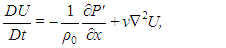
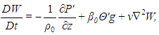
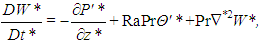
Accepting the validity of the Boussinesq approximation, the equations for mass, momentum and energy conservation in a two-dimensional domain are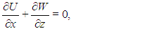 | (1) |
 | (2) |
 | (3) |
 | (4) |
in which U and W are respectively the horizontal and vertical components of velocity (in the x- and z-directions), t is the time,  and
and  represent respectively the fluid density and bulk expansion coefficient values right above the bottom plate,
  and
and  denote respectively the fluid kinematic viscosity and thermal diffusivity,
  and
and  are respectively the pressure and temperature fluctuations with respect to the reference hydrostatic state, g stands for the acceleration of gravity module, and
  is the temperature difference between the plates spaced of a distance H. The material derivative is written as D()/Dt, and
 indicates the two-dimensional laplacian.The actual temperature and pressure field can be recovered by adding the reference state to the fluctuations. In the case of temperature, it consists of the linear profile
 | (5) |
where  is the constant temperature at the bottom plate.In order to obtain dimensionless equations, characteristic length, time and temperature scales are chosen to be H,
  and
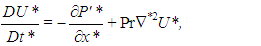
and  . Denoting non-dimensional variables with an asterisk, we have
 | (6) |
 | (7) |
 | (8) |
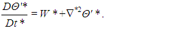 | (9) |
In equations (7)–(9),  is the non-dimensional material derivative (moving with the dimensionless velocity field), and
  is the dimensionless laplacian. As usually occurs when one nondimensionalizes fluid mechanics equations, two dimensionless parameters arise: the Prandtl number Pr, which is the ratio between the fluid momentum and thermal diffusivities, and the Rayleigh number
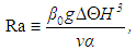 | (10) |
accounting for the ratio between buoyancy and viscosity forces acting on a fluid parcel. The Reynolds number increases with increasing Ra. Therefore, Ra is also a measure of the intensity of turbulence within the flow. The functional relationship between these two dimensionless parameters is subject of active research, [9] being a well-known scaling theory for it.At last, it is possible to reduce the number of equations and variables by defining a non-dimensional stream function  such that
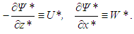 | (11) |
Moreover, the pressure can be eliminated by cross-differentiating equations (7) and (8) and taking the difference between the results. Using the definition of the stream function above, we end up with a set of two equations and two variables: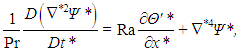 | (12) |
 | (13) |
2.2. Boundary Conditions
In RBC, there are no boundaries in the x-direction, given that the domain is infinite in this direction. Thus, it is only necessary to apply adequate boundary conditions at the plates, that is, at z*=0 and z*=1. Firstly, both plates are impermeable, so that W* vanishes at these positions. Since this is valid for all x*, one can write | (14) |
In the case of the horizontal component of velocity, it must be observed that, in order to obtain the Lorenz system, it is necessary to apply shear-free boundary conditions at the plates. This means that it is not U* that vanishes at the plates, as it would happen if no-slip conditions were applied, but its derivative with respect to z*. In terms of the stream function, | (15) |
Together, (14)–(15) cause the laplacian of the stream function (which equals minus the vorticity) to vanish at the plates.Furthermore, one expects that, at least in a temporal average, there is no net mass flux crossing a vertical section of the domain, since there is nothing forcing the flow horizontally, as it would be the case if there were a pump imposing a horizontal pressure gradient, for example. Because the discharge (per unit of cross-sectional area) between two streamlines is given by the difference between the corresponding values of the stream function, this assumption leads to the fact that  must have the same value at both plates’ inner surfaces. Since the stream function is defined in terms of its derivatives, its absolute value has no physical meaning, so that we can set
 | (16) |
at the plates.As for the temperature field, in view of the fact that the plates temperatures are maintained constant by external heating/cooling, there is no temperature fluctuation at the boundaries. Hence, | (17) |
2.3. Fourier Series and Lorenz Equations
In [1], Saltzman proposed to expand the stream function and the temperature fluctuations into double Fourier series in space, allowing their respective coefficients to vary in time. He proved that, for both variables, the trigonometric (real-valued) form of these series satisfying the boundary conditions is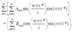 | (18) |
When he substituted truncated series of this form for the stream function and temperature fluctuations in (12)–(13), Saltzman obtained a system of ordinary differential equations for the coefficients, which he solved numerically. Most coefficients approached zero after a transient period, and for some simulation conditions, only three of them did not vanish. In [7], Lorenz argued that this same behavior would have been obtained if only these three coefficients had been included since the beginning.Using the same argument, we propose the highly truncated Fourier representations: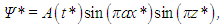 | (19) |
 | (20) |
in which A, B and C are functions to be determined of time alone, and a is the horizontal wavenumber, so that the wavelength is 2a-1. The velocity components are obtained by differentiating the stream function: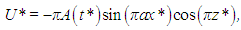 | (21) |
 | (22) |
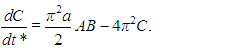
Substituting (19)–(20) into (12)–(13) and equating the terms multiplying the same functions of x* and z*, we obtain the set of non-linear equations known as the Lorenz system: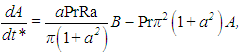 | (23) |
 | (24) |
 | (25) |
The coefficients A, B and C and the time t* differ from the variables used by Lorenz in [7] by scaling factors. However, they were kept in this form due to its greater proximity with the physical variables. A much more detailed derivation of the Lorenz system can be found in [10].In the present study, this system was numerically solved using a standard fourth-order Runge-Kutta algorithm implemented in Fortran 95, departing from random initial conditions. Substitution of the numerical results into the Fourier series (20)–(22) allowed mean profiles and heat fluxes, for instance, to be obtained. As in [7], we let the Prandtl number be constant and equal to 10. The Rayleigh number was varied in order to obtain different flow regimes, as discussed next.
2.4. Thermal Instability Considerations
As deduced in [4], and also well explained in [11], the onset of convection happens when the Rayleigh number exceeds the critical value | (26) |
The corresponding horizontal wavenumber is | (27) |
When the Rayleigh number is below this critical value, perturbations on the hydrostatic equilibrium decay and this condition is stable. When the Rayleigh number is above it, perturbations grow and convection currents develop. Inspired by this, we define the parameter | (28) |
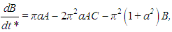
which is greater than unity in unstable conditions.For moderate values of r, the solutions to the Lorenz equations correspond to steady convection, a situation in which convection cells of fixed shape occur. However, as it is demonstrated in [7], if r is set to beyond the second critical value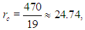 | (29) |
steady-state solutions become unstable themselves, and the Fourier series coefficients oscillate permanently.
2.5. Computation of Means and Dimensionless Fluxes
We assumed that the ergodic hypothesis is true for the Lorenz system, so that expected values could be computed as time averages of sufficiently long series.The kinematic heat flux by conduction can be obtained from Fourier’s law: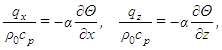 | (30) |
where qx and qz are the x- and z-components of the heat flux density (per unit of cross-sectional area), and cp is the specific heat at constant pressure of the medium. In terms of the dimensionless variables used before, 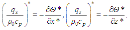 | (31) |
The Fourier series (20), however, gives the non-dimensional fluctuation of temperature with respect to the reference state. To relate this quantity to the heat flux by conduction, it is necessary to use the dimensionless form of equation (5) to obtain the actual temperature profile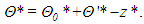 | (32) |
Substituting this in equation (31) leads to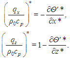 | (33) |
The dimensionless advective heat fluxes in the x- and z- directions are respectively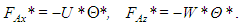 | (34) |
Using equation (32), one is able to write them in terms of temperature fluctuations,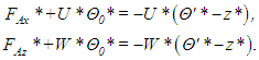 | (35) |
The terms including the temperature of the bottom plate were placed on the left side, since they are divergence-free due to (6). Hence, they represent a background heat advection that does not affect the energy balance of any imaginable control volume.Finally, the dimensionless turbulent heat fluxes in the horizontal and vertical directions are simply | (36) |
where  denotes the expected value and the lower-case letters represent turbulent fluctuations, that is, fluctuations around the expected value.
3. Static Regime
3.1. Time Series and Phase Spaces
Figure 1 shows the solution of the Lorenz equations for r = 0.8 as a function of time. The small random perturbations initially imposed rapidly decay and all coefficients tend asymptotically to zero. Observing equations (20)–(22), one can notice that when A, B and C are zero, there is no motion or temperature fluctuations, which means that the static condition occurs. Therefore, the numerical solution of the Lorenz system agrees with the results predicted by the stability theory for RBC.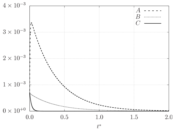 | Figure 1. Time series of Lorenz’s coefficients for r = 0.8. Perturbations decay and hydrostatic equilibrium is recovered |
Figure 2 illustrates the same solution projected on the A-B plane of phase space. The trajectory described by the solution of the Lorenz system always ends at the origin, regardless of the point where it starts. This characterizes the origin as an attractor for all r < 1. Naturally, this can be seen in other projections of phase space as well.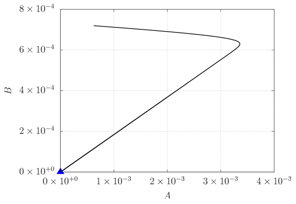 | Figure 2. Projection of the trajectory described by the solution of the Lorenz system on the A-B plane in phase space for r = 0.8. The origin (blue triangle) is an attractor whenever r < 1 |
3.2. Mean Profiles and Heat Fluxes
When r < 1, once the steady-state is reached, the velocity field is zero and so are the temperature fluctuations. Hence, the dimensionless temperature profile is the linear profile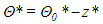 | (37) |
for all x*.In this situation, the turbulent and advective fluxes are all zero. As for the molecular heat flux, its horizontal component vanishes and its vertical component equals unity.
4. Steady Convection
4.1. Time Series and Phase Spaces
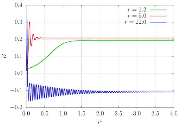
Figures 3–5 show the solution of the Lorenz equations for some values of r in the interval 1 < r < rc as a function of time. All coefficients attain steady-state values, even though the transient period has a variable duration with r. Differently from what happened for r < 1, these steady-state values are non-zero, indicating the permanent presence of motion and temperature fluctuations. | Figure 3. Time series of A for 1 < r < rc. One of two alternative steady-state values A∞(r) is reached in each simulation |
 | Figure 4. Time series of B for 1 < r < rc. One of two alternative steady-state values B∞(r) is reached in each simulation |
 | Figure 5. Time series of C for 1 < r < rc. There is only one possible steady-state value C∞(r) which is reached in each simulation |
In fact, these values can be analytically determined by setting the time derivatives to zero in (23)–(25). This procedure leads to the three critical points of the Lorenz system, P1, P2 and P3, whose coordinates (A,B,C) in phase space are respectively (0,0,0), (A∞,B∞,C∞) and (-A∞,-B∞,C∞), where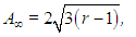 | (38) |
 | (39) |
 | (40) |
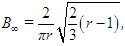
P1 is an attractor for r < 1, unstable otherwise. For 1 < r < rc, P2 and P3 become attractors. Whether one or the other is reached depends on the initial condition and on truncation errors caused by the numerical solution. The latter are capable of deviating trajectories in phase space due to chaos, which originates from the non-linearities present in the Lorenz system.Notice that P2 and P3 only differ by the sign of the first two coefficients. In RBC, this corresponds to convective cells having different senses of rotation. Furthermore, the intensity of convection increases with increasing values of the Rayleigh number, since A∞ given by equation (38) (and therefore the velocity field) is a growing function of r.Figure 6 shows two example trajectories described by the solutions of the Lorenz system in phase space for r = 5 and r = 22. They both leave from close to the origin, but one of them is attracted by P2, whereas the other is attracted by P3. It can be noticed that the larger the value of r, the longer it takes for the trajectory to approach the attractor. Moreover, the position of the attractors depends on the Rayleigh number. | Figure 6. Two trajectories corresponding to different Rayleigh numbers projected on the B-C plane in phase space. P1 (the origin) is represented by a blue triangle, whereas P2 corresponds to the two points on the right (one for each value of r) and P3 to the two points on the left |
4.2. Mean Profiles and Heat Fluxes
Figure 7 illustrates the steady-state flow for r = 22. As all figures in this section, it shows the situation in which the solution was attracted to P2 (all coefficients have positive values). Both the velocity and temperature field are easily obtained by substituting the steady-state coefficients (38)–(40) into the Fourier series (20)–(22). The dimensionless temperature deviation from its value at the bottom plate is represented by colors, and varies from zero (at z* = 0) to –1 (at z* = 1). The trajectories of fluid particles, which can be inferred from the velocity field, are closed, being similar to a pattern known as roll-convection.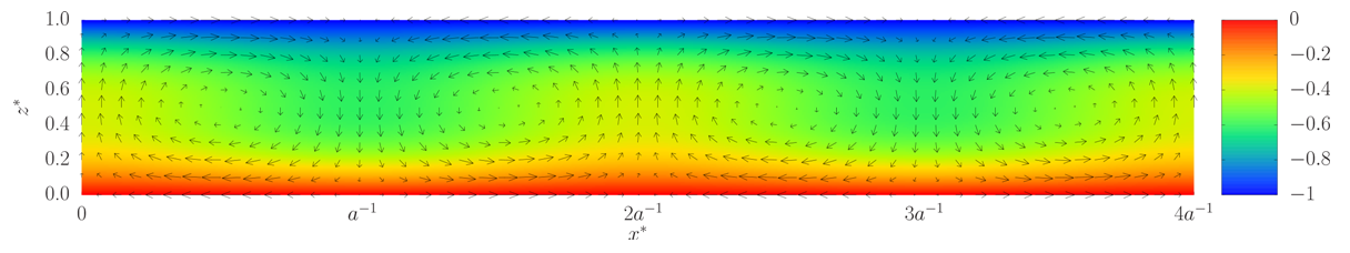 | Figure 7. Dimensionless temperature field (colors), expressed in terms of deviation from the temperature of the bottom boundary, and velocity field (vectors) for r = 22 |
We can notice ascending currents warming the medium and descending currents cooling it periodically in x*. According to [7], B is proportional to the temperature difference between ascending and descending currents, and similar signs of A and B indicate that warm fluid is rising and cold fluid is descending. This is in agreement with the steady-state solution obtained, in which A∞ and B∞ always have the same sign.Figures 8 and 9 show the vertical profile of the horizontal and vertical (respectively) components of velocity for r = 22. These images make clear that the boundary conditions are respected, since U* has a null gradient at the boundaries, it integrates to zero between the plates (so that there is no net discharge) and W* vanishes at the plates. Both profiles vary in module and sign as x* changes. Figure 8 refers to a position in which sin(πax*) in (21) is unity, and figure 9 refers to a position in which cos(πax*) in (22) is unity, so that both profiles here represented contain the maximum value of each velocity component. U* is greatest at the positions z* where W* is zero, and vice-versa. Also, U* attains greater values than W*.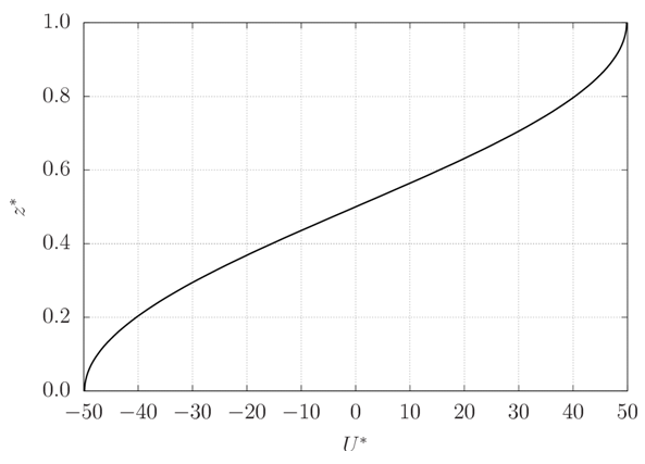 | Figure 8. Vertical profile of the horizontal component of velocity (r = 22) |
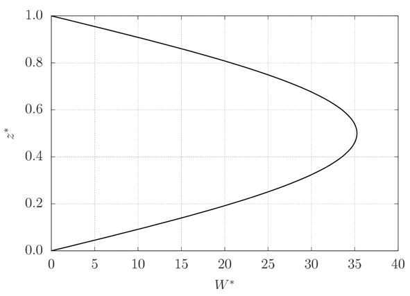 | Figure 9. Vertical profile of the vertical component of velocity (r = 22) |
In figure 10 were represented three temperature profiles, corresponding to x*-positions in which fluid is uniquely rising, sinking or moving horizontally. In all cases, temperature tends to be homogenized away from the plates. This mean temperature equals the average between the temperatures of the plates at positions in which the flow is purely horizontal. That mean temperature is slightly superior to this average at positions in which warm fluid is rising, and slightly inferior to it where cold fluid is sinking. The strong gradients near the plates characterize the formation of thermal boundary layers. Again, this is in agreement with [7], according to whom positive values of C, which is proportional to the departure of the temperature profile from linearity, indicate the presence of important gradients near the boundaries. Indeed, the steady-state values C∞ are always positive.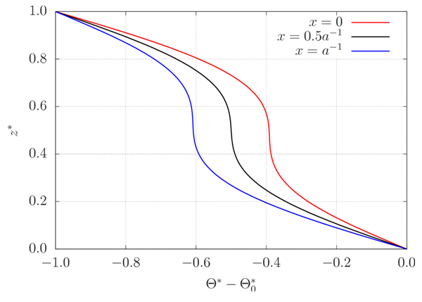 | Figure 10. Vertical profiles of the temperature deviation from the bottom plate temperature for r = 22. The red profile corresponds to positions in which warm fluid is only rising, the blue one to positions in which cold fluid is only sinking, and the black one to positions where motion is horizontal |
Figure 11 illustrates heat conduction for positions of ascending, descending and horizontal currents. Evidently, conduction is strongest near the boundaries, where the gradients are most important. It falls almost to zero at the intermediate position z* = 0.5, where the temperature is almost uniform. Also, notice that the vertical component of heat conduction is always positive, since the temperature decreases monotonically with z*.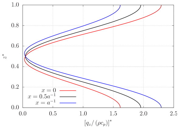 | Figure 11. Vertical profile of vertical heat conduction for r = 22. The red, blue and black profiles correspond respectively to positions of ascending, descending and horizontal currents |
At positions of ascending currents, the temperature falls slowly with z* near the bottom plate, but falls rapidly with z* near the upper plate. This leads to more intense heat conduction near the latter. At positions of descending currents, the opposite happens; temperature falls rapidly at the bottom and slowly at the top, and heat conduction is more important near the bottom. At positions of horizontal currents, heat conduction is symmetric with respect to z* = 0.5.Heat conduction in the horizontal direction is much smaller than it is in the vertical direction. This can be seen by observing figure 7 and remembering that the vector representing the conductive heat flux is always perpendicular to isotherms (points having the same color in figure 7), which are either approximately horizontal or considerably spaced, indicating weak gradients.The vertical profile of heat advection in the vertical direction is shown in figure 12. Its module is larger far from the boundaries, and it changes signs and its shape depending on the horizontal position. In the horizontal direction, heat advection is much greater than conduction.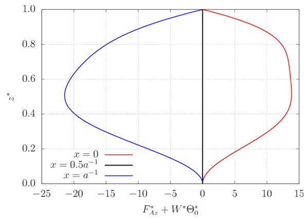 | Figure 12. Vertical profile of vertical heat advection for r = 22. The red, blue and black profiles correspond respectively to positions of ascending, descending and horizontal currents |
Finally, figures 13 and 14 compare the profiles of heat advection and conduction in the vertical direction at positions of ascending and descending currents. Conduction is always positive, and its magnitude is much smaller than that of advection. Nevertheless, it is the most important heat transfer mechanism near the boundaries, where the steepest temperature gradients take place and vertical advection of heat is weak due to the no-penetration condition. This is similar to what happens in the CBL [2]. The maximum values of total heat transfer occur very close to z* = 0.5 at positions of descending currents, whereas it happens nearer the upper plate at positions of ascending currents. | Figure 13. Vertical profile of vertical heat conduction and advection for r = 22 at a position of ascending currents |
 | Figure 14. Vertical profile of vertical heat conduction and advection for r = 22 at a position of descending currents |
5. Chaotic Solutions
5.1. Time Series and Phase Spaces
Figures 15–17 illustrate time series of the three coefficients for three different values of r > rc. In this case, none of them attains a steady-state, and they keep oscillating. This happens due to the fact that both the hydrostatic condition and the steady convection become unstable at high Rayleigh numbers. In phase space, this means that none of the three critical points P1, P2 and P3 is stable; there is no point attractor for r > rc. | Figure 15. Time series of A for r > rc |
 | Figure 16. Time series of B for r > rc |
 | Figure 17. Time series of C for r > rc |
It can be seen that, for increasing r, the amplitude of oscillation of A increases, whereas those of B and C decrease. In addition, for slightly supercritical r, the solutions to the Lorenz system are clearly non-periodic; they never repeat themselves [7, 12]. However, for larger values of r, they seem to change less through time, as if they were approaching periodic solutions. The frequency of oscillation of all coefficients increases with increasing r. The velocity components are proportional to A, and the temperature fluctuations are linear combinations of B and C at each point of the flow, so that the behavior of the physical quantities is similar to that of the coefficients.The solutions to the Lorenz equations are well known for being chaotic, which means they are extremely sensitive to initial conditions due to their non-linear nature. Indeed, even running numerical simulations of the Lorenz system using different time steps leads to different time series due to amplification of round-off errors. However, numerical solutions affected by chaos are also solutions to the Lorenz system by virtue of a property known as shadowing, according to which there exists an initial condition corresponding to the solution obtained as well [12]. This justifies the use of a unique time step in this study (Δt* = 10-4).The chaotic solution of the Lorenz equations for r > rc is somehow analogous to what would be a turbulent regime in RBC, since turbulence is also unpredictable due to its non-linear character. In this sense, we call the quantities in equation (36) “turbulent” fluxes, even though RBC is a two-dimensional problem (therefore it cannot be turbulent) and the Lorenz equations are not an exact solution to RBC.Figures 18–20 show phase space projections corresponding to the time series presented in figures 15–17. Regardless the initial conditions imposed, the solution to the Lorenz system always converges to the same region of the phase space, forming a structure of fractal dimension known as the Lorenz attractor [12]. Therefore, if one considers the solutions of the Lorenz equations as being random processes, their statistics, such as the expected value, must not depend on the initial conditions, even though the processes themselves are highly dependent on them.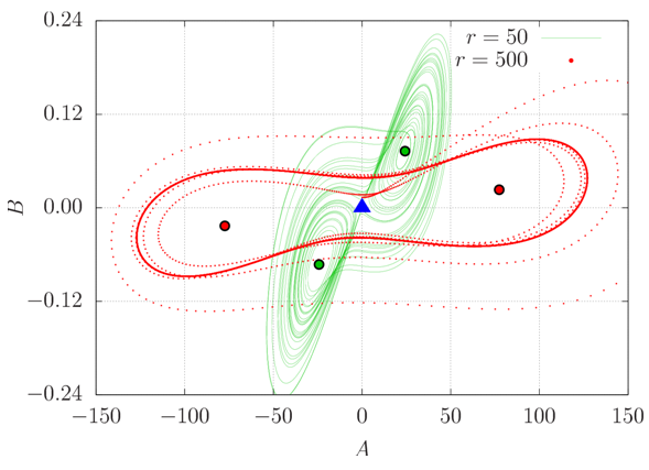 | Figure 18. Phase space projected in the A-B plane for two supercritical values of r. The blue triangle indicates the position of the origin, whereas the two pair of large dots indicate the foci of the attractors |
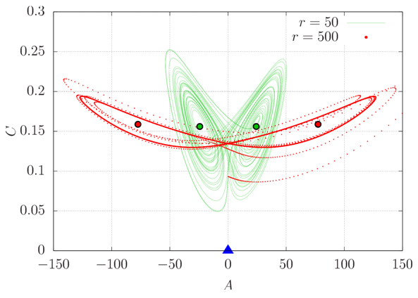 | Figure 19. Phase space projected in the A-C plane for two supercritical values of r. The blue triangle indicates the position of the origin, whereas the two pair of large dots indicate the foci of the attractors |
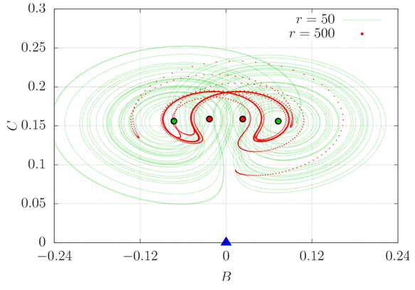 | Figure 20. Phase space projected in the B-C plane for two supercritical values of r. The blue triangle indicates the position of the origin, whereas the two pair of large dots indicate the foci of the attractors |
It can be seen in figures 18–20 that the shape of the attractors depends on the Rayleigh number. In reality, the solution orbits around two foci whose positions are those corresponding to steady convection for r < rc, given by equations (38)–(40), and represented by large dots in the figures. It is possible, for instance, to analytically determine the slope S of a line in the A-B plane passing through both foci to have an idea of the slope of the attractor itself. It is | (41) |
a monotonically decreasing function of r, tending to zero as r tends to infinity. In projections of phase space containing the C axis, the slope is not a function of r due to the fact that C∞ has only one sign. Besides, as r tends to infinity, (A∞, B∞, C∞) tends to (∞,0,(2π)-1).For large values of r (small red dots in figures 18–20), the solution seems to converge to a unique trajectory, which agrees with the fact that the time series in figures 15–17 appear to become periodic. However, this is only an impression and does not happen; the solution never repeats itself exactly [12]. Trajectories in phase space become closer and closer, but do not collapse into a single one.
5.2. Autocorrelation Functions and Integral Time Scales
The autocorrelation function measures the correlation of a process with itself in the future, being a measure of how long it takes for the process to “forget its past”. For a statistically stationary random process A(t), it is defined as [5]: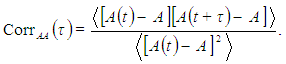 | (42) |
Numerically, it can be computed as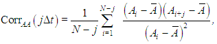 | (43) |
 | (44) |
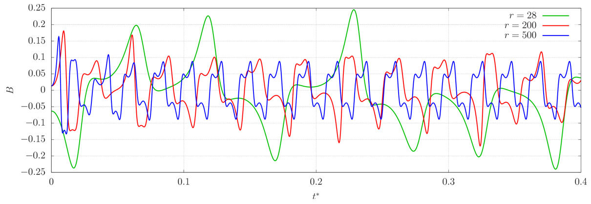
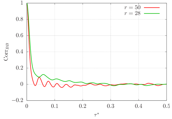
with  Another important measure is the integral of the autocorrelation function from 0 to infinity, known as the integral time scale, which equals half the time necessary for a process to have effectively zero correlation with itself.For subcritical r, there exist stationary solutions, so the processes A, B and C never lose their memories. Therefore, the autocorrelation functions of A, B and C were computed only for supercritical values of r. This was done using a time series of dimensionless duration equal to 400, the data from first dimensionless time being was suppressed to avoid any influence of the initial conditions. The result is shown in figures 21–23 for r = 28 and r = 50. It can be seen that the autocorrelation function is well-behaved for A and B, since it rapidly tends to zero, indicating that both variables lose their memories quite quickly. The small-amplitude oscillation that persists in both autocorrelation functions for larger values of time lag is due to the fact that time series of finite duration were used to compute them.
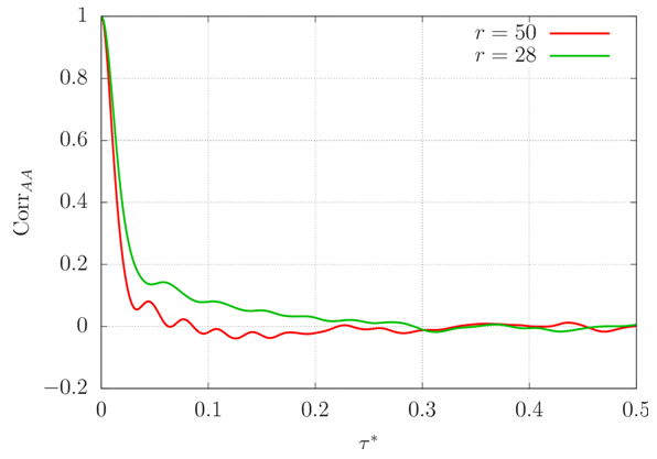 | Figure 21. Autocorrelation function of A for two supercritical values of r |
 | Figure 22. Autocorrelation function of B for two supercritical values of r |
 | Figure 23. Autocorrelation function of C for two supercritical values of r |
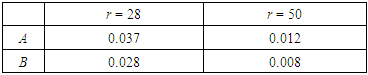
The integral time scales of A and B are shown in table 1. In this range of values for r, the integral time scale of both variables decreases with larger r. Besides, B decorrelates with itself faster than A does.Table 1. Integral time scale of A and B for some values of r
 |
| |
|
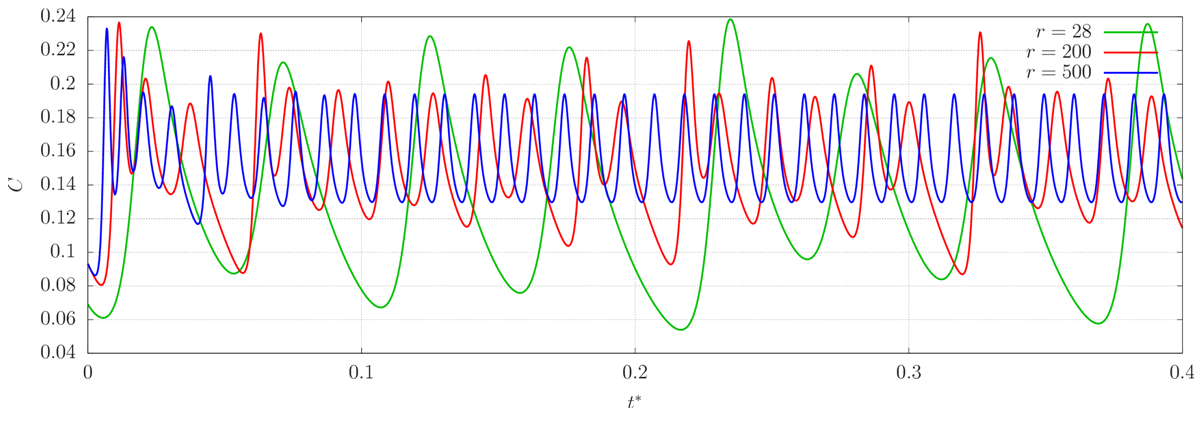
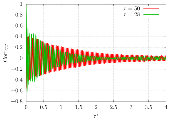
The autocorrelation function of C, however, is much different from those of A and B. It oscillates a lot before tending to zero, and takes considerable time to do so. For greater values of r, convergence is even slower. In reality, due to the fact that the solution of the Lorenz system approaches a periodic solution as r increases, the autocorrelation functions of all three variables tend to be periodic for large r. As a consequence, the integral time scale of any variable does not exist, in practice, for large r. The autocorrelation functions of the three variables are shown in figure 24 for r = 200 as an example of this situation.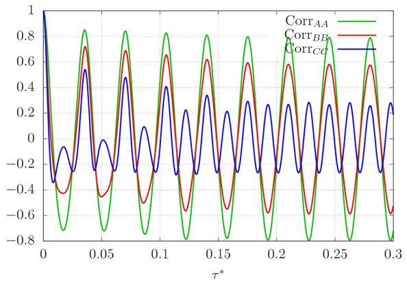 | Figure 24. Autocorrelation function of the three coefficients for r = 200 |
The autocorrelation functions (and integral time scales) of the velocity components are identical to those of A, since U* and W* consist of this random process multiplied by a constant (with respect to time), which is incapable of changing the quantities considered. The temperature fluctuations, however, are different linear combinations of the random processes B and C at each point of the domain. Hence, their autocorrelation functions were computed as well, and they revealed to have very similar behavior to that of C, regardless the position of the flow considered.
5.3. Mean Profiles and Heat Fluxes
The mean values of the coefficients were computed as the average of 1000 realizations of the Lorenz system starting from different random initial conditions. Each realization had a dimensionless duration equal to 20, which is sufficient to span a fair number of integral time scales.For all r > rc, the expected values of A and B are zero. Thus, the mean values of U* and W* are also zero, since the velocity field changes signs continuously, so that the solution can orbit around both foci of opposite signs in phase space. Interpreting B as the temperature difference between ascending and descending currents, as explained in [7], this result indicates that the fluid mean temperature is homogenized in the horizontal direction.C is the only coefficient having non-zero mean. Actually, the C-coordinate of the attractor’s foci in phase space has only one sign, so that the time series of C always oscillates above zero. A natural question that arises is whether the mean value of C equals C∞ given by equation (40). As it can be seen in figure 25, the answer is no. However, the mean of C is a growing function of C∞, and this relation can be modelled, for instance, by the power law: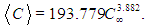 | (45) |
This adjustment has a coefficient of determination of 0.91, and is represented by the black curve in figure 25. The adjustment is also illustrated in figure 26 as a function of r.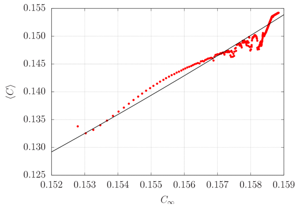 | Figure 25. Expected values of C in function of C∞ obtained from the numerical solution of the Lorenz system (red dots) and adjusted power-law (black line) |
Notice in figure 26 that the expected value of C seems to asymptotically approach a finite value as r grows (a smaller value than (2π)-1 to which tends C∞ though). Assuming that this trend continues to be valid for greater values of r, it can be inferred that the mean values of the coefficients appearing in the Lorenz system become independent of the Rayleigh number as it tends to infinity. Interpreting C as the departure of the temperature profile from linearity [7], its increasing values with increasing r indicate stronger temperature gradients near the plates.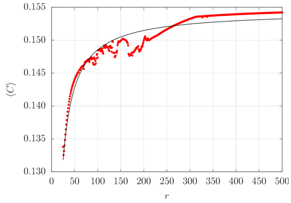 | Figure 26. Expected values of C in function of r obtained from the numerical solution of the Lorenz system (red dots) and modelled by equation (45) (black line) |
The mean value of the temperature fluctuations is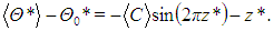 | (46) |
As happens to the velocity field, the mean temperature field becomes independent of the horizontal position x*. This happens due to the sign switching of A and B. In the chaotic regime, all temperature profiles are very similar to the black profile in figure 10. In the CBL, flow properties can be homogenized in the horizontal directions due to the displacement of the ascention and subsidence centers of the convective cells.The independence of conduction of heat of the horizontal direction follows immediately from the fact that the temperature field is not a function of x*. Indeed, the mean of the horizontal component of heat conduction is zero. As for the vertical component, we have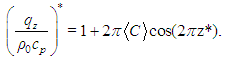 | (47) |
Considering other heat transfer mechanisms, it is important to notice that simply taking the mean of equations (35) gives birth to both heat transport by mean advection and by turbulence. The first is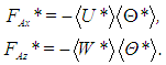 | (48) |
However, the means of both velocity components vanish, so that mean advection vanishes as well.At last, to calculate the turbulent fluxes, notice that | (49) |
Due to the fact that the mean velocity field is zero. All variables in the right-hand side of equation (49) can be directly obtained from the Fourier series (20)–(22). Hence, the turbulent fluxes depend on the quantities  and
and  . The numerical result is that they are
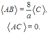 | (50) |
The same result is analytically obtained by taking the mean of the Lorenz system (23)–(25) assuming statistical stationarity. Therefore, the turbulent fluxes are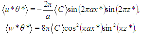 | (51) |
uniquely depending on the mean value of C. These are the only statistics variable in x* in the chaotic regime. Notice that the vertical turbulent heat transfer is always positive.The vertical molecular and turbulent heat transfer profiles for r = 500 are shown in figure 27 for a position in which vertical turbulent heat transfer is maximum. Conduction is greatest near the plates, where important temperature gradients take place, and smaller away from it, where the temperature varies little with z*. Notice that, if the expected value of C attained (2π)-1 (limit to which tends C∞), vertical conduction of heat given by (47) would vanish at z* = 0.5, indicating locally homogeneous temperature. Turbulent heat transport vanishes at the plates due to the boundary conditions, and is greatest at z* = 0.5.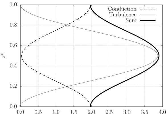 | Figure 27. Profiles of vertical heat transfer by conduction and turbulence (both always positive), for a position at which the turbulent transport is maximum |
6. Conclusions
Although the Lorenz system results from highly truncated Fourier series representing the stream function and the temperature fluctuations, employing it to describe the steady-state or mean behavior of RBC for different Rayleigh numbers led to meaningful results, which agree qualitatively with results from fully developed turbulence in micrometeorology.It was found that chaos, analogously to turbulence, tends to homogenize flow properties such as the temperature. In addition, the asymptotic behavior of the solution as r tends to infinity becomes independent of r. Finally, conduction was found to be the most important heat transfer mechanism near the bottom plate, turbulence and advection being more important at higher levels, similarly to what happens in the CBL.Many results could be obtained analytically due to the relative mathematical simplicity of the Lorenz system. However, its solutions are probably more and more different from RBC as r grows, since the non-linearities of the flow produce more Fourier modes that must be included to represent faithfully all important phenomena happening in a truly turbulent flow.
ACKNOWLEDGEMENTS
The authors wish to acknowledge all those who contributed to this study.
References
| [1] | Saltzman, B., 1962, Finite amplitude free convection as an initial value problem, Journal of the Atmospheric Sciences, 19(4), 329–341. |
| [2] | Stull, R. B., 2012, An Introduction to Boundary Layer Meteorology, Springer Science & Business Media. |
| [3] | Bénard, H., 1900, Étude expérimentale des courants de convection dans une nappe liquide. Régime permanent: tourbillons cellulaires, Journal de Physique Théorique et Appliquée, 9(1), 513–524. |
| [4] | Rayleigh, L., 1916, On convection currents in a horizontal layer of fluid, when the higher temperature is on the under side, The London, Edinburgh, and Dublin Philosophical Magazine and Journal of Science, 32(192), 529–546. |
| [5] | Pope, S. B., 2000, Turbulent Flows, Cambridge University Press. |
| [6] | Davidson, P. A., 2004, Turbulence: an Introduction for Scientists and Engineers, Oxford University Press. |
| [7] | Lorenz, E. N., 1963, Deterministic nonperiodic flow, Journal of the Atmospheric Sciences, 20(2), 130–141. |
| [8] | Danforth, C. A., 2001, Why the weather is unpredictable, an experimental and theoretical study of the Lorenz equations, honor thesis. |
| [9] | Grossmann, S., and Lohse, D., 2000, Scaling in thermal convection: a unifying theory, Journal of Fluid Mechanics, 407, 27–56. |
| [10] | Rodakoviski, R. B., 2016, Análise da correlação entre escalares no problema de Rayleigh-Bénard por meio das equações de Lorenz, honor thesis. |
| [11] | Chandrasekhar, S., 1970, Hydrodynamic and Hydromagnetic Stability, Dover Publications. |
| [12] | Motter, A. E., and Campbell, D. K., 2013, Chaos at fifty, Physics Today, 66(5), 27–33. |

 Abstract
 Reference
 Full-Text PDF
 Full-text HTML