-
Paper Information
- Paper Submission
-
Journal Information
- About This Journal
- Editorial Board
- Current Issue
- Archive
- Author Guidelines
- Contact Us
American Journal of Environmental Engineering
p-ISSN: 2166-4633 e-ISSN: 2166-465X
2018; 8(3): 45-53
doi:10.5923/j.ajee.20180803.01

Precipitation and Runoff Modelling in Megech Watershed, Tana Basin, Amhara Region of Ethiopia
 Abstract
 Reference
 Full-Text PDF
 Full-text HTML
Afera Halefom1, Ermias Sisay1, Tesfa Worku2, Deepak Khare2, Mihret Dananto3, Kannan Narayanan3
1Department of Hydraulic and Water Resources Engineering, Faculty of Technology, Debre Tabor University, Ethiopia
2Department of Water Resources Development and Management, Indian Institute of Technology Roorkee, India
3Department of Water Supply and Environmental Engineering, Institute of Technology, Hawassa University, Hawassa, Ethiopia
Correspondence to: Kannan Narayanan, Department of Water Supply and Environmental Engineering, Institute of Technology, Hawassa University, Hawassa, Ethiopia.
| Email: |  |
Copyright © 2018 The Author(s). Published by Scientific & Academic Publishing.
This work is licensed under the Creative Commons Attribution International License (CC BY).
http://creativecommons.org/licenses/by/4.0/

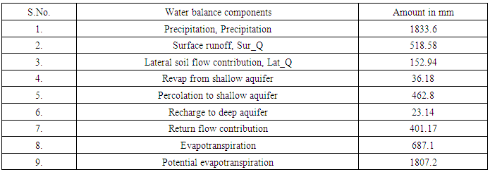
This study examined applicability and performance of SWAT model for the catchment of Megech watershed in Tana basin located in Amhara region of northern Ethiopia. Calibration and validation of runoff process has been done on monthly basis for the periods 1984-2004 and 2005-2014. Trend of rainfall in 35 years has been done using the Mann-Kendall trend test. Analysis of water balance showed that base flow is 52% of the total discharge in the Megech watershed that contributes more than surface runoff. Total surface runoff of Megech watershed is about 48% of the total and 37% of losses in the watershed through the evapotranspiration. The result indicated that there has been good agreement between simulated and observed flow. Therefore, the model performance has been applicable and strong predictive capability for the Megech watershed. According to Mann-Kendall trend test, during short rainy season substantial decreasing trend was observed in all the stations. Likewise, during the long rainy season increasing trend was recorded. It can be concluded that on the annual scale, the trend of rainfall during the study periods have shown a decreasing trend with lower variability of rainfall distribution.
Keywords: SWAT, Calibration, Validation, Mann-Kendal trend test, Watershed modelling
Cite this paper: Afera Halefom, Ermias Sisay, Tesfa Worku, Deepak Khare, Mihret Dananto, Kannan Narayanan, Precipitation and Runoff Modelling in Megech Watershed, Tana Basin, Amhara Region of Ethiopia, American Journal of Environmental Engineering, Vol. 8 No. 3, 2018, pp. 45-53. doi: 10.5923/j.ajee.20180803.01.
Article Outline
1. Introduction
- Ethiopia, often referred to as the water tower of East Africa, is dominated by the mountain landscape, and precipitation-runoff processes on the mountains is the source of surface water for a large part of Ethiopia (Derib 2009), therefore, understanding of rainfall-runoff processes is critical to erosion and increase agricultural productivity (Tesfa and Tripathi 2016). The majority of the sedimentation of rivers in the basin takes place during the early period of the rainy season and the sediment peaks are consistently measured before recovery peaks for a given rainy season (Steenhuis et al. 2009; Halefom et al., 2017). GIS and Remote Sensing has applied in Debre-Mewi watershed, Ethiopia, to identify soil erosion mapping and hotspot area. Soil erosion was calculated through overlay analysis, which ranged from 0.0046 to192 tons/ha/year, (Mulatie et al. 2011). SWAT model was used to model soil erosion, identify soil erosion-prone areas and assess the impact of best management practices on sediment reduction in the Blue Nile basin. The model results showed that a satisfactory agreement between daily observed and simulated sediment concentrations as indicated by Nash-Sutcliffe efficiency greater than 0.83 (Betrie et al. 2011). Setegn et al (2010) applied SWAT model in the Lake Tana Basin, Ethiopia. The evaluation of the model did satisfactorily for stream flows prediction and shows that there is a good agreement between the measured and simulated flows that was verified by coefficients of determination and Nash-Sutcliffe coefficient greater than 0.5. In addition to this, more than 60% of loss in the watershed is through evapotranspiration. Shiferaw et al. (2016) used SWAT model to assess the impact of climate change on surface hydrological processes in the Omo-Gibe river basin, Ethiopia. The evaluation of the model indicates that a good performance during the Calibration (NSE=62.6%, R2=72.4% and D=14.37%), and Validation (NSE=68%, R2=68.1% and D=4.57%). In addition, the annual potential evapotranspiration shown increasing trend for future climate change scenarios. Khare et al. (2015), applied SWAT model for the assessment of Surface Runoff in a Barinallah Watershed. Assefa et al. (2010), assessed soil erosion rates under actual farming conditions by measuring the dimensions and the number of rills in 15 agricultural fields in Debre-Mewi watershed near the Lake Tana, Ethiopia. The annual rill erosion rate was 8 to 32 t ha-1. Greatest rates of erosion occurred at planting early in the season but became negligible in August.SWAT is a physically based model, developed to predict the impact of land-management practices on water, sediment, and agricultural chemical yields in watersheds with varying soil, land use, and management conditions (Neitsch et al. 2012). SWAT can simulate hydrological cycles, vegetation growth, and nutrient cycling with a daily time step by disaggregating a river basin into sub-basins and hydrologic response units (HRUs). HRUs have lumped land areas within the sub-basin comprised of a unique land cover, soil, and management combinations. This allows the model to reflect differences in evapotranspiration and other hydrologic conditions for different land cover and soil (Neitsch et al. 2012). SWAT has been applied in the highlands of Ethiopia and demonstrated satisfactory results (Easton et al. 2010; Setegn et al. 2010; Betrie et al. 2011). The SWAT model requires spatial, temporal and management data to model the hydrology of a watershed.The Tana Basin is part of the Blue Nile Basin, which is characterized by increased demand for water for agriculture, industry, households and electricity generation. No effective measures have been taken to combat flood, soil erosion, and sedimentation problems. Lack of decision support tools and limiting of the data on the desired scales based on soil and land use based on hydrology and topography, and weather are factors that significantly hinder the research and development in this area. As a result, the sub-basin requires proper planning and management of water. Megech is one of the watersheds that drain into the sub-basin of Lake Tana. Due to the increasing demand for water mainly for irrigation under great pressure and growing population, which is no longer practiced today and water is mainly used for domestic and pastoral purposes. The continuous increase of population growth demand more land for cultivation and therefore more forest has exposed to deforestation consequently accelerate runoff and sedimentation (Meshesha et al. 2016; Worku et al. 2017). In addition, the increasing uncertainty of the availability of surface water and increasing water pollution are threatening the social and economic development. Megech watershed has experienced visible symptoms of soil degradation in the form of soil erosion and sedimentation of the Megech River. This paper mainly focused on investigating runoff generation considering climate trend analysis of Megech Watershed, Ethiopia.
2. Material and Methods
2.1. Description of Study Area
- The Megech watershed is located in the northern part of the Lake Tana sub-basin in Amhara region of Ethiopia. It originates near the Simien Mountains at an altitude of around 4000 m. The total watershed is 663 km2 at the lake inlet of which 500 km2 is gauged. The lake catchment lies between latitude 12°30'45" to 7°43'0' N, and longitude 37°21'34"-37°35'26"E. In 1997, a dam was constructed on a tributary of Megech River that supplies the town of Gondar with water. The reservoir has a surface area of 51 ha and a design capacity of 5.3 Mm3 with a catchment area of 68 km2 (i.e., 13% of the gauged). Eighty-two percent of the catchment has slopes of more than 8%. Ninety-five percent of the catchment is cropland and Eutric and Leptosols cover about 82% of the area. In 2007, one-third of the volume of the reservoir was filled with sediment due to high soil erosion from the catchment.
2.2. Hydrological Modelling
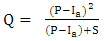
- SWAT model is operation, conceptual and physical based model that operate on the daily time step. The objectives in the model development was in order to predict the runoff, climate change, sediment yield and land use change in the catchment (Arnold and Fohrer 2005; Gassman et al. 2007). Process of model development is presented in Fig 1. The model can be used to analyse small or larger catchments by representing them into different sub-basins, which are subdivided into Hydrological Response Units (HRUs) with homogenous land use, slope and soil types. The model is embedded within Arc GIS and integrated various spatial environmental data including information about soil features, land cover, weather and topographic features. To simulate runoff volume and sediment yield SWAT model required data for like soil data, weather data and land use map (Haverkamp et al. 2005; Neitsch et al. 2005). SWAT model simulate the hydrological cycle on the basis of the following subsequent water balance equation:
 | (1) |
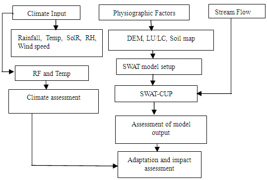 | Figure 1. Conceptual framework of methodology |
 | (2) |
 | (3) |
 | (4) |
 | (5) |
2.3. Model Calibration and Validation
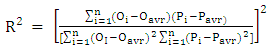
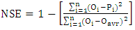
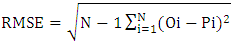
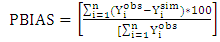
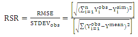
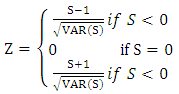
- The focus of validation and calibration result of the model is on improving the performance of SWAT model at each station. For runoff and sediment yield, the actual values for each measured time interval has compared along with the simulated result for the same time interval. In this regard, the whole runoff and sediment graph has fitted by SWAT.Coefficient of determination (R2), the Nash and Sutcliffe (1970) model efficiency coefficient (NSE), the Root Mean Square Error (RMSE), percentage bias (PBAIS) and observation standard ratio (RSR), determine simulation of SWAT model result accuracy. The value of R2 is the indicator of strength of linearity relationship between actual and simulated values. The value of R2 ranged between 0.0 to 1.0 and therefore, the higher the value, the better is agreement. Whereas, the NSE simulation result indicates how well the plot of actual values against simulated values fits the 1:1 line. The value of R2 is obtained by using the following equation:
 | (6) |
 | (7) |
 | (8) |
 | (9) |
 | (10) |
2.4. Model Inputs
- The spatial distributed data needed for the analysis of ArcSWAT interface includes Digital Elevation Model (DEM), land use, soil data and weather data. In addition, the river discharge data are used for the calibration and validation analysis.
2.4.1. Digital Elevation Model
- Digital Elevation model (DEM) used as input for SWAT hydrological model. For this study, high grid resolution raster DEM data (30x30m) will be obtained from the USGS databases of the SRTM (Shuttle Radar Topography Mission) website (http://earthexplorer.usgs.gov/). In the SWAT model, DEM is used to delineate the watershed and generate the drainage pattern and associated physiographic attributes. This was done by embedded in ArcGIS10.3.
2.4.2. Soil Type
- Different soil textural and physico-chemical properties for various soil layers of each soil type in the watershed are required by SWAT model. Here, Soil map can show the spatial distribution of the different types of soils texture in the watershed. In this study the soil data collected from the Food and Agricultural Organization (FAO, 1996), which provides the Digital Soil Map of the World (DSMW). This connected with a database containing the soil’s characteristics such as soil texture, hydrological soil group’s, available water content, hydraulic conductivity, so on.
2.4.3. Weather Data
- The weather data used for the analysis of hydrological water balances are minimum and maximum air temperature, precipitation, relative humidity, wind speed and solar radiation for the period of 1984-2014. Meteorological data engaged in this study acquired for two purposes. First is the data used as input for SWAT model to determine the water balance component of the watershed. Second is the data used for climate change scenario in the watershed by using Mann-Kendall.
2.4.4. River Discharge
- The data used for the calibration and validation are daily river discharge of Megech river. Hydrological data, available stream flow data of the basin gauging station required for calibrating and validating SWAT hydrological model. Hence the gauging stations of entire watershed which have continuous record for a relatively long period and therefore average monthly stream flow discharge data for these stations collected.
2.4.5. Land use
- LULC data have also a significant effect on the hydrological modelling. Therefore, a detail analysis and mapping of the LULC is crucial for proper hydrological modelling. It affects the runoff and sediment transport in the watershed. For this study, the LULC map (Fig 2) is extracted through the processing of satellite Landsat 8 image which is downloaded from USGS database website (http://earthexplorer.usgs.gov/) that has a spatial resolution of 30 m. The unsupervised classification in ERDAS IMAGINE 2014 is done to reclassify the land use of the area which used for the HRUs analysis.
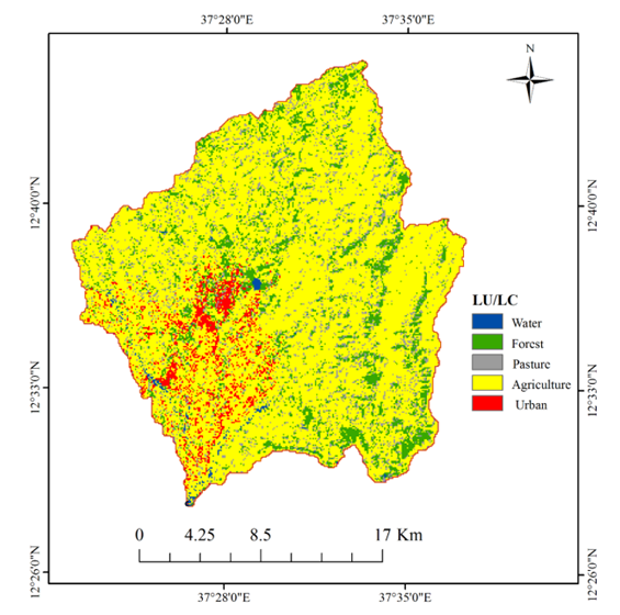 | Figure 2. LU/LC of the study area |
2.5. The Mann–Kendall Trend Analysis
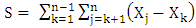
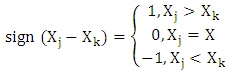
- Trend of temperature refers to an increase or decrease of variables through time. The Mann-Kendall trend test is a statistical test, which is widely used applicable method in order to analyse the spatial and temporal variation of trend in temperature and rainfall in a prolonged time series (Yue and Wang 2004). The Mann –Mann (1945) has formulated Kendall test, it is a non-parametric test used to detect the trend, and Kendall (1975) has given distribution of test statistic. The idea of the Mann- Kendall (MK) test is in order to assess statistically is there is increasing or decreasing trend variables over time. In order to perform the trend analysis, sequential order data should be required. Initially fix the sign of the sample result (the difference between series consecutive sample results). Sign (Xj-Xk) is used to show the function of resulted in the values 1, 0 or -1 on the basis of Xj- Xk, in which j > k, the function is computed as follows:
 | (11) |
 | (12) |
 | (13) |
 | (14) |
 | (15) |
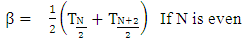
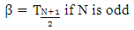
2.6. Sen’s Slope Estimator
- The slope of linear trend in a time series was estimated by using non-parametric methods developed by Sen (1968). The slope of time series trend is obtained by the following equation;
 | (16) |
 | (17) |
 | (18) |
3. Results and Discussion
3.1. Sensitivity and Uncertainty Analysis
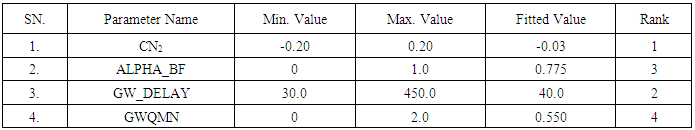
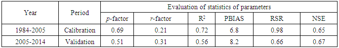
- The result for simulation, which has expressed by using 95 percent prediction uncertainties (95PPU), usually cannot be comparable with the observation signals using R2, NSE and RSR statistics. Therefore, according to Abbaspour et al. (2007), r-factor and p- factor measurement have been suggested. The p-factor is referred to as the percentage of measured data, which is bracketed by 95PPU. The value of p-factor is 1, which inferred 100% bracketing of the actual data, therefore indicating correct simulation process. Whereas, r-factor is used to measure the calibration quality and which specifies the thickness of 95PPU. The lower value of r-factor (~0) shows lower uncertainty bound of prediction. Generally, the value of p-factor and r- factor is used to confirm the power of uncertainty assessment and model calibration (Shuol et al. 2006). The essential sensitive parameters for calibration and simulation are listed (Table 1 & 2).
|
|
3.2. Model Calibration and Validation
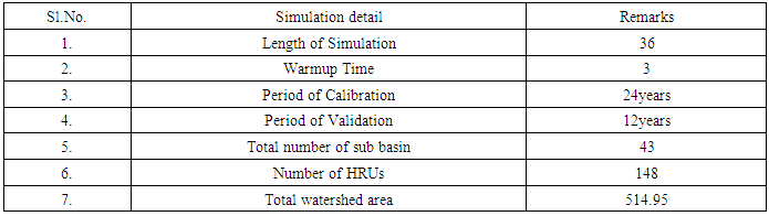
- Model is used to show the near reality of actual natural system. For this study the statistical test and graphical representation have been used for the model calibration and validation. The model was calibrated and validated by using SUFI-2 (Sequential Uncertainty Fitting-2). The calibrated and validated result of the model have been done using observed stream flow in time series for stream gauging stations (Table 3), the result indicated that good model performance for the catchment (Fig. 3). During the calibration periods (1984-2004), the value of R2 was obtained 0.72, while the same periods, the Nash-Sutcliffe efficiency (NSE) during monthly flow calibration result registered as 0.65. The value of measured and observation standard ratio (RSR) is 0.98, the percentage bias (PBIAAS) is 6.8% (Table 3).On the other hand, the result during validation process for the period 2005-2014, the value of coefficient of determination (R2) is 0.56. Whereas, for the same periods the value of NSE (Nash-Sutcliffe Efficiency) for the monthly flow has been shown 0.67, RSR (measured and observation standard ratio) is 0.66, and PBIAS (percentage bias) is 8.6% (Table 3).
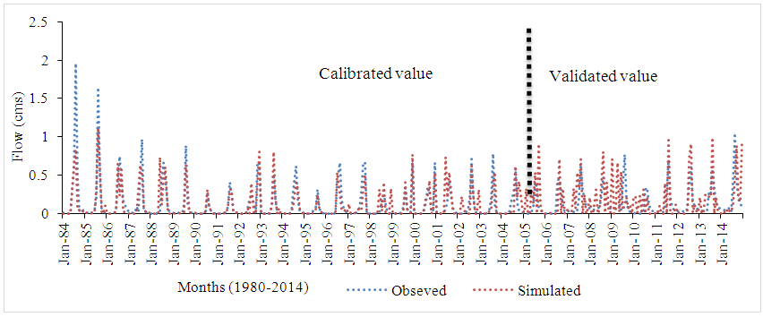 | Figure 3. Calibration and validation result of Runoff processes |
|
|
3.3. Rainfall Trend Analysis of Megech Catchment
- Climatic variables were analysed for the Belg season, Kermit season, Bega season and annual scale using MK trend test. The results of the trend test was derived for all the climatic variables and compared at the 5% level of significance. The test statistics (S) and Zmk obtained from three different season and annual scale as shown in Table 5 for both levels of significance (significant and insignificant). The positive value of Zmk statistics confirmed that the increasing trend whereas the negative values Zmk indicated the decrease of climatic variables. After having MK test, the Sen’s estimator of slope was done in order to obtain the change per unit of the observed trend throughout the time series of the climatic variables in each seasons and annual scale.
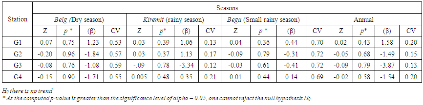 | Table 5. Rainfall Trend analysis |
4. Conclusions
- In this study process scale Soil and Water Assessment Tools (SWAT) model integrated with the Arc GIS interface Arc SWAT as well as Sequential Uncertainty Fitting (SUFI-2) calibration and validation procedures have effectively employed to model and quantify runoff process on a monthly time- step in the Megech watershed of Ethiopia. SUFI-2 parameter calibration and validation of runoff process has been successfully performed. The result confirmed that there has been good agreement between the predicted and observed runoff process at the watershed outlet. MK test and Sen’s slope estimates have been conducted to estimate the long-term trend of rainfall for the study watershed. The MK test statistic and Sen’s estimator observed both positive and negative trends in the annual and seasonal rainfall. Based on the results obtained, all stations annual and seasonal rainfall trends were found to be decreasing with varied magnitude, which infers the trend of climate change needs an urgent response in order to reduce vulnerability of the community to climatic shock. Based on the current observation, SWAT results and MK trend test have produced useful information to recommend soil and water conservation management practice in the erosion and degradation prone highland area of Ethiopia. The output of the study shall be used for the preparation of watershed management strategies for sustainable land and water resources management in the Nile Basin.